ACU-T: 3600 Melting of Diesel Exhaust Additive within an Enclosed Tank
This tutorial provides the directions for setting up, solving, and post-processing results for a simulation that models the approximated melting of the common diesel fuel exhaust additive that is contained within a notional tank. Prior to starting this tutorial, you should have already run through the introductory tutorial, ACU-T: 1000 Basic Flow Set Up, and have a basic understanding of HyperWorks CFD and AcuSolve. To run this simulation, you will need access to a licensed version of HyperWorks CFD and AcuSolve.
Problem Description
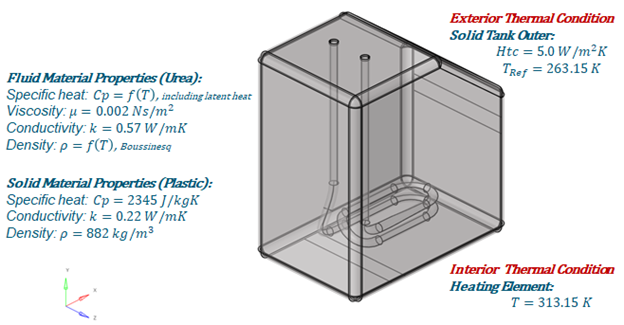
Figure 1.
Start HyperWorks CFD and Open the HyperMesh Database
-
From the Home tools, Files tool group, click the Open Model tool.

Figure 2.The Open File dialog opens.
Validate the Geometry
The Validate tool scans through the entire model, performs checks on the surfaces and solids, and flags any defects in the geometry, such as free edges, closed shells, intersections, duplicates, and slivers.
Figure 3.
Set Up Flow
Set Up the Simulation Parameters and Solver Settings
-
From the Flow ribbon, click the Physics tool.

Figure 4.The Setup dialog opens. -
Under the Physics models setting:
- Set Time marching to Transient.
- Set the Time step size to 0.5 seconds.
- Set the Final time to 600.0 seconds (10 minutes).
- Select Spalart-Allmaras as the Turbulence model.
- Activate Include Gravitational Acceleration and set it to [0.0, -9.81, 0.0] m/s2.
- Set the Pressure scale to Absolute.
- Active Heat transfer.
- Set the Temperature scale to Absolute.
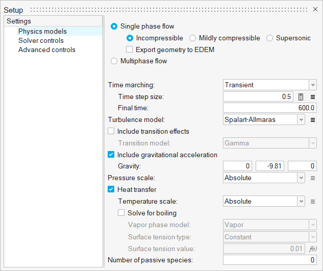
Figure 5. -
Under the Advanced controls setting:
- Select Modify flow stagger settings.
- Assign Maximum flow stagger settings to 4 iterations.
- Select Modify temperature stagger settings.
- Assign Maximum temperature stagger settings to 6 iterations.
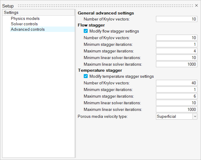
Figure 6.
Assign Material Properties
-
From the Flow ribbon, click the Material Library tool.

Figure 7. -
Click
 to create a new material.
-
Name the material Urea, set the density (ρ) type to
Boussinesq and enter Density (kg/m3) and
Reference temperature (K) values as shown below.
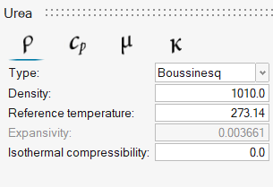
Figure 8. -
Click
 three times to add three rows to the table and then
enter the table values according to the figure below.
three times to add three rows to the table and then
enter the table values according to the figure below.
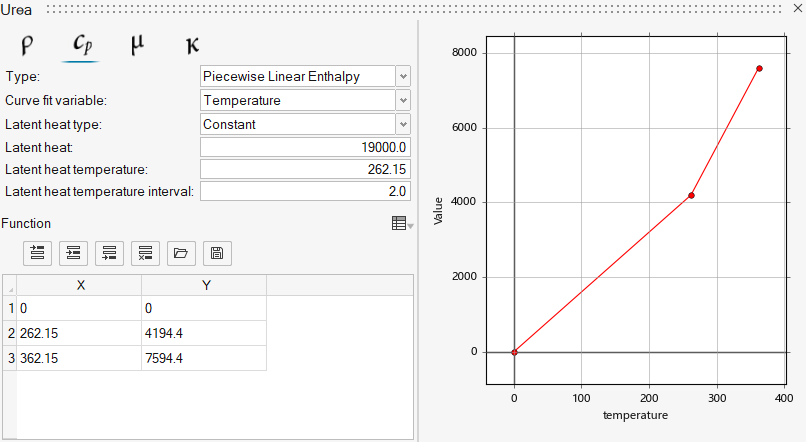
Figure 9. -
Select the My Materials tab then click to
create a new material.
-
Specify two solid material properties for Plastic and
Copper using the figure below.
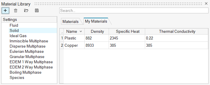
Figure 10. -
From the Flow ribbon, click the Material tool.

Figure 11. -
Assign the Solid material – Plastic – to the outer tank volume and the Fluid
material – Urea – to the inner tank volume, as shown in the figure below.
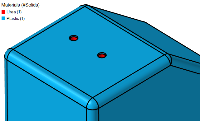
Figure 12.
Define the Porous Medium
-
From the Flow ribbon, Porous
tool group, click the Cartesian Porous Media tool.

Figure 13. -
Assign the Porous Media values according to the following figure.
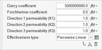
Figure 14. -
Click
 besides Effectiveness type.
-
In the new dialog, click four time to add four empty rows to the table then
enter values according to the figure below.

Figure 15. -
On the guide bar, click
 to execute
the command and exit the tool.
to execute
the command and exit the tool.
Assign the Flow Boundary Conditions
-
From the Flow ribbon, click the No Slip tool.

Figure 16. -
Select the exterior faces of the plastic tank.
Select a single face then right-click and choose . This selects all faces that are connected by shared edges.
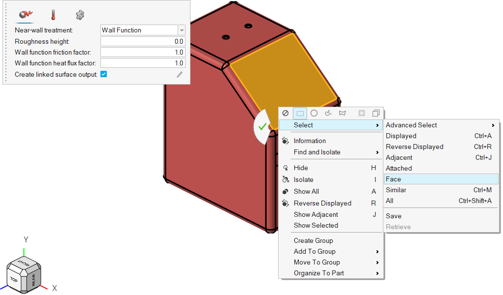
Figure 17. -
Set the Convective heat reference temperature to 263.15
K.
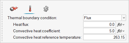
Figure 18. -
On the guide bar, click
 to execute the command and remain in the
tool.
to execute the command and remain in the
tool.
-
Change the Thermal boundary condition to Temperature and
set the Temperature (K) to 313.15.
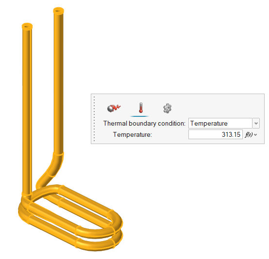
Figure 19. -
Click
 on the guide bar.
-
From the Flow ribbon, click the Thin tool to define a virtual thin
solid.

Figure 20. -
In the microdialog, set the layer thickness (m) to
0.002 and the Material to
Copper.
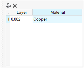
Figure 21. -
Click on the guide bar.
-
From the Flow ribbon, click the arrow next to the
Setup tool set, then select Parameters.
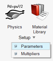
Figure 22.The Parameter Manager opens. -
Assign variables associated with the problem definition to compute the mesh
settings, including the diameter of the heating element
(d_line), the number of elements across the diameter
(n), the local surface mesh size
(dx), the volume mesh size
(dx_vol), and the first layer height
(flh).
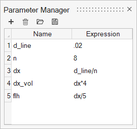
Figure 23.
Generate the Mesh
-
From the Mesh ribbon, click the Surface tool.

Figure 24. -
In the legend, right-click on Heating Element (34),
select Edit, and verify that the average element size of
Heating Element is set to dx.
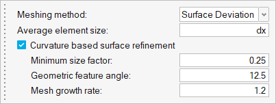
Figure 25. -
Click the Boundary Layer
tool.

Figure 26. -
In the legend, right-click on BL_Active (66), select
Edit, and verify that the values in the following
figure.
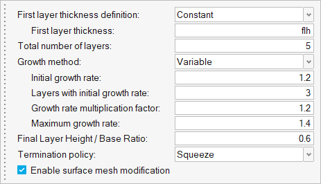
Figure 27. -
Click the Volume Mesh
tool.

Figure 28. -
Define the Solid volume mesh parameters as in the
following figure, where dx_vol=0.015m.
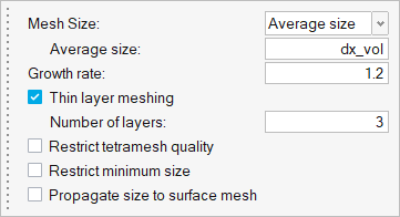
Figure 29. -
Define the Fluid volume mesh parameters as in the
following figure.
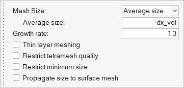
Figure 30. -
Click the Volume tool.

Figure 31. -
Define the mesh operations as shown in the following figure.
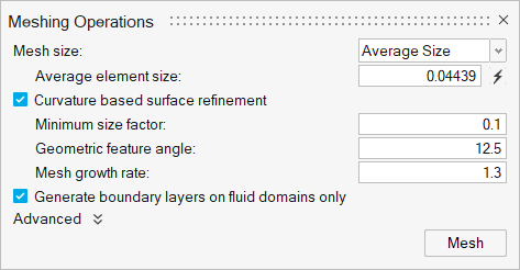
Figure 32.
Define a Surface Monitor and Run AcuSolve
-
Form the Solution ribbon, click the Surfaces tool.

Figure 33. -
Select by Face after selecting a single face on the interior tank walls.
This will select all faces that are shared.
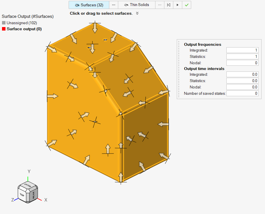
Figure 34. -
On the guide bar, click
to execute
the command and exit the tool.
-
From the Solution ribbon, click the Run tool.

Figure 35.The Launch AcuSolve dialog opens. -
Set the Default initial conditions as in the following figure.
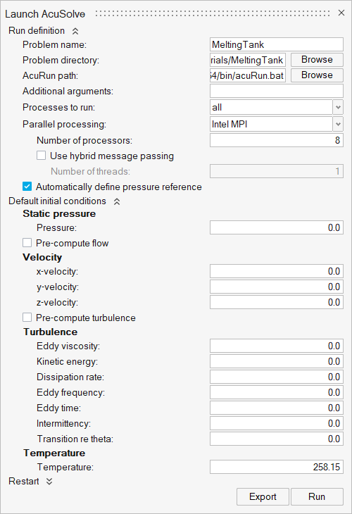
Figure 36.
Post-Process the Results
Post-Process with the Plot Tool
-
From the Solution ribbon, click the Manage tool.

Figure 37. -
In the Run Status dialog, right-click on the AcuSolve run and select Plot time
history to launch the Plot Manager.
The residual and solution ratios for pressure, velocity, eddy viscosity, and temperature are shown.
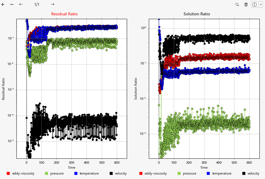
Figure 38. -
Select the Wall – Output to plot the heat flux entering
the domain from the heating element.
Note: The value stabilizes near the end of the simulation, indicating that the model is approaching the prescribed thermal boundary conditions.
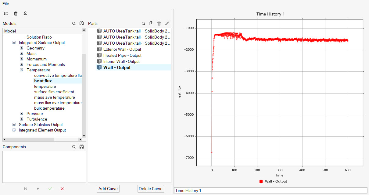
Figure 39. Integrated heat flux entering the domain from the heating element surface -
Select the Interior Wall – Output to plot the
temperature increase of the inside wall of the tank.
Note: The value is not stabilized by the end of the simulation, indicating that the model has not reached the final temperature to balance the prescribed thermal boundary conditions. After 10 minutes of physical time, approximately 35% of the additive has been melted.
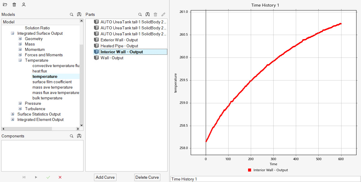
Figure 40. Integrated temperature on the interior surface of the tank wall
Post-Process with HyperWorks CFD Post
-
From the Post ribbon, click the Boundary Groups
tool.

Figure 41. -
Click
 on the guide bar to open the
Advanced Selection dialog.
on the guide bar to open the
Advanced Selection dialog.
-
Select Exterior_Wall - Output then close the
dialog.
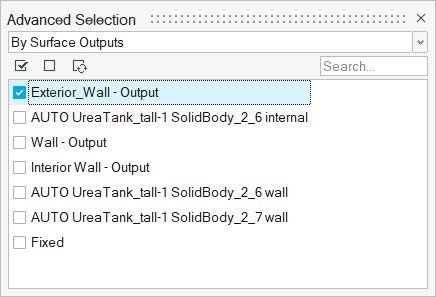
Figure 42. -
On the guide bar, click
to execute
the command and exit the tool.
-
From the Post ribbon, click the Iso-Surfaces tool.

Figure 43. -
Select temperature as the Iso Variable and set the Iso
Value of temperature (K) to 261.15.
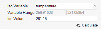
Figure 44. -
In the display properties microdialog, define the
Display as constant and select a color of choice.
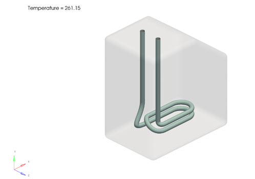
Figure 45. Transparent boundary of the tank, showing an Iso-Surface of temperature T=261.15 K, Time=0.0 sec -
Using the results animation toolbar, skip to the end of the simulation
results.
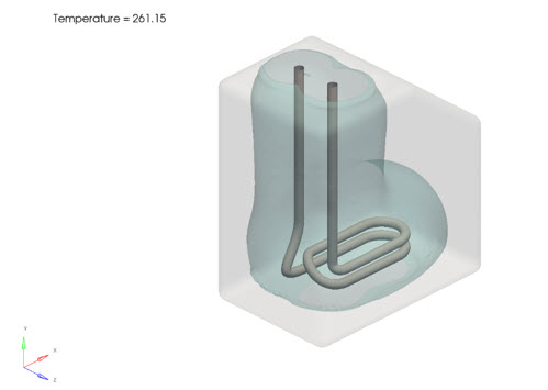
Figure 46. Transparent boundary of the tank, showing an Iso-Surface of temperature T=261.15 K, Time=600.0 sec
Summary
In this tutorial, you learned how to set up and solve a flow and thermal simulation with temperature dependent porous media effectiveness. Utilizing the proposed implementation allowed you to specify the melting point of a fluid and compute the melted region of the fluid. You started by importing the HyperWorks CFD input database and then you defined the porous medium to control the melting point of the fluid. Next, you assigned the thermal boundary conditions and generated the mesh using the parametric variable definitions. Once the solution was computed, you created a plot of the heat flux and temperature for the critical surfaces with the model using HyperWorks CFD Plot Manager.