Pareto Plot Post Processing

Plot the Effects of Variables on Responses in Hierarchical Order

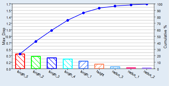
Rank the effects of input variables on output responses in hierarchical order (highest to lowest) in the Pareto Plot post processing tab.

From the Post Processing step, click the Pareto Plot tab.
Using the Channel selector, select the response to plot.

Tip: Analyze multiple responses simultaneously by switching the Multiplot option to (multiple plots) and selecting the responses to plot using the Channel selector.
Analyze the pareto plot.

The effect of input variables on output responses is indicated by bars. Hashed lines with a positive slope indicates a positive effect. If an input variable increases, the output response will also increase. Hashed lines with a negative slope indicates a negative effect. Increasing the input variable lowers the output response.

A line represents the cumulative effect.

Configure the pareto plot's display settings by clicking

(located in the top, right corner of the work area). For more information about these settings, refer to Pareto Plot Tab Settings.

Pareto Plot Tab Settings

Settings to configure the plots displayed in the Pareto Plot post processing tab.

Access settings from the menu that displays when you click

(located above the Channel selector).

Effect curve: Show line to represent the cumulative effect.
# Top factors displayed: Specify the number of input variables (bars) displayed in the plot.
Note: This settings does not change the calculated effects.
Multivariate Effects: Calculate the effect using all input variables simultaneously.
Linear Effects: Calculate the effect using each input variable independently.; For more information about linear effects, refer to Linear Effects Post Processing.
Include Interactions: Include first order, two way interactions along with first order effects, and calculate interactions consistently with the choice of linear or multi-variate effects.; For more information about interactions, refer to Interactions Post Processing.
Exclude dependent/linked inputs: Only show the independent input variables.
Tip: Excluding dependent/link inputs reduces redundant information.

Multivariate Effects

Calculate the effect using all input variables simultaneously.

Multivariate effect of an input variable is the difference between the output response values when the variable is at its lower and upper values while the remaining variables are held constant. All calculations are based on a single linear regression model including all variables.

Example

A system with two variables, X and Y and the output response, F (X,Y).

Table 1. Design Matrix
Run	X	Y	F (X, Y)
1	42.0	108.0	1385.4
2	54.0	156.0	2290.2
3	66.0	84.0	3421.2
4	78.0	132.0	4778.3
5	32.4	165.6	824.4
6	44.4	93.6	1548.3

$F (X, Y) = A+B*X+C*Y$ is the reference regression model and intercept. A and coefficients, B and C, are calculated using the data set above.

A = - 2609.8

B = 88.6

C = 2.5

Regression equation:

F (X, Y) = -2609 .8 + 88 .6*X + 2 .5*Y

Effect of X (lower = 32.4, upper = 78.0)
Since we are investigating the effect of X only, Y is held constant. For this example, use the mean value ( $\bar{Y}$ = 123.2).

X = 32.4, Y = 123.2

$F (32.4, 123.2) = - 2609.7937 + 88.6056 * 32.4 + 2.4841 * 123.2 = 567.0787$

X = 78, Y = 123.2

$F (78, 123.2) = - 2609.7937 + 88.6056 * 78 + 2.4841 * 123.2 = 4607.4948$

$Δ F = 4607.4948 - 567 .0787 = 4040.4161$
Effect of Y (lower = 84, upper = 165.6)
Since we are investigating the effect of Y only, X is held constant. For this example, use the mean value ( $\bar{X}$ = 52.8).

X = 52.8, Y = 84

$F (52.8, 84) = - 2609.7937 + 88.6056 * 52.8 + 2.4841 * 84 = 2277.2536$

X = 52.8, Y = 165.6

$F (52.8, 165.6) = - 2609.7937 + 88.6056 * 52.8 + 2.4841 * 165.6 = 2479.9623$

$Δ F = 2479.9623 - 2277.2536 = 202.7087$

Input Variable	Multivariate Effect
X	4040.4161
Y	202.7087