Learn how to generate a 1000 Hz plus 3000 Hz sinusoidal wave with additive noise,
apply a Chebyshev Type II filter, compute a Fast Fourier Transform (FFT) and power spectral
density, display simulation results in a vector scope, and downsample the output of a
buffer.
Files for This Tutorial
filterPSD.scm
A finished version of the models you build in the tutorials along with any files
required to complete the tutorials are available at this location:
<installation_directory>/tutorial_models/.
Generating a Sinusoidal Wave with Additive Noise
Create a model and define a diagram context for a sinusoidal wave with additive
noise.
On the ribbon, select New
Model, then Save Model.
In the dialog that appears, enter the path to your working directory with the
file name: filterPSD_practice.scm.
From the Palette Browser, add the following blocks into the
modeling window:
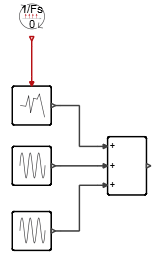
From Activate > SignalGenerators, drag 1 SampleClock block, 1
Random block, and2
SineWaveGenerator blocks.
From Activate > MathOperations, drag 1 Sum block.
For each block: double-click the block, enter the parameter values as
indicated, then click OK.
On the Sum block, double-click, and for Number of
inputs, enter: 3; for all Input Ports, enter:
"+" .
Block
Define Parameter
SampleClock
Sample period:
1/Fs
Random
Distribution:
Normal
SineWaveGenerator
(1)
Frequency:
2*pi*1000
SineWaveGenerator
(2)
Frequency:
2*pi*3000
Sum
Number of inputs:
3
For all Input Ports:
"+"
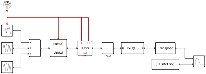
Connect the blocks and adjust the links like this:
On the ribbon, select the Diagram tool .
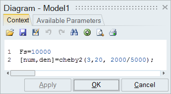
On the Context tab, enter: Fs = 10000, and click
Apply.
Applying a Chebyshev Type II Low Pass Filter
Apply the OML function, Cheby2, in a diagram context.
The Cheby2 function generates the coefficient of the transfer function of the low pass
filter.
On the ribbon, select the Diagram tool .
On the Context tab, enter the command:
[num,den]=cheby2(3,20,2000/5000);
This command generates the coefficient of the transfer function of the low
pass filter, which has an order of 3, a cut-off frequency of 2000 Hz, and a stop
band attenuation of 20 dB. The returned variables num and
den are used as coefficients of the numerator and
denominator of a discrete transfer function representing the
filter.
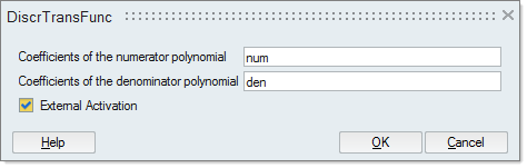
From the Palette Browser > Activate > Dynamical, drag 1 DiscrTransFunc block into the
diagram.
On the DiscrTransFunc block, double-click, and enter
these parameter values:
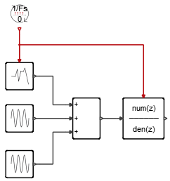
Connect the blocks so that the sine wave with additive noise passes through the
digital low pass filter implemented with a discrete transfer function:
Computing the FFT and Power Spectral Density
Define blocks in your model to compute the Fast Fourier Transform and Power Spectral
Density.
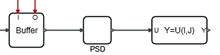
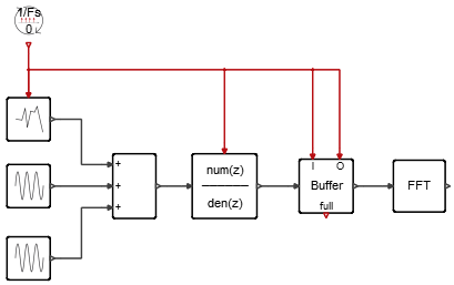
From the Palette Browser > Activate > Buffers, drag 1 Buffer block into the
diagram.
On the Buffer block, double-click. In the block dialog,
for length, enter: N.
From the Palette Browser > Activate > MatrixOperations, drag 1 FFT block into the diagram.
Connect the blocks like this:
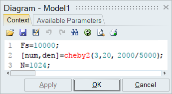
On the ribbon, select the Diagram tool .
On the Context tab, enter the variable: N=1024.
This variable specifies for 1,024 points of data to be sampled and sent to
the FFT block.
Note: The one-sided power spectral density is computed with the
equation P= 2 ∗ |ff |
^
2/(F∗N)
From the Palette Browser > Activate > MathOperations, drag 1 Abs and 1
Power block into the diagram.
On the Power block, double-click. In the block dialog,
for power, enter: 2.
From the Palette Browser > Activate > MathOperations, drag 1 Gain block into the diagram.
On the Gain block, double-click. In the block dialog,
for Gain, enter: 2/ (Fs*N).
Connect the blocks like this:
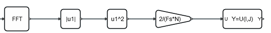
From the Palette Browser > Activate > MatrixOperations, drag 1 MatrixExtractor block into the
diagram.
On the MatrixExtractor block, double-click, enter the
following parameter values, and click OK:
For Index vector I, select : (all), which is the
default.
For Index vector J, select Defined as parameter,
and enter [1:N/2+1].
Select One-based indexing.
Connect the blocks like this:
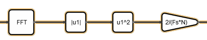
Click and drag your mouse left to right to box-select the blocks
FFT, Abs,
Power, and Gain.
With the blocks selected, from the ribbon, click, Create Super
Block.
In the tree of the Property Editor, under General, click the field for
Name, and enter PSD.
The super block reflects the new name:
Displaying Results with a VectorScope Block
View simulation results in a power spectrum density graph.
From the Palette Browser, add the following blocks into
your diagram:
From Activate > MatrixOperations, drag 1 Transpose block.
From Activate > SignalViewers, drag 1 VectorScope block.
From Activate > SignalGenerators, drag 1 Constant block.
On the Constant block, double-click. In the block
dialog, for the parameter Constant, enter
[0:Fs/N:Fs/2]', and click OK.
On the VectorScope block, double-click. From the block
dialog, select the box for External X Value and
Plot after simulation ends, and click
OK.
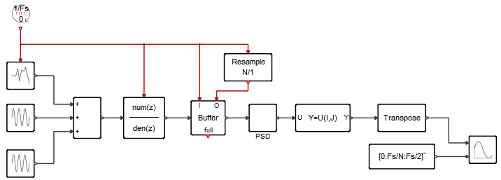
Assemble and connect the blocks like this:
On the ribbon, select Run.
Double-click the VectorScope block.
The VectorScope window appears displaying a plot of the simulation
results. To fit the view of the plot into the window, middle-mouse click.
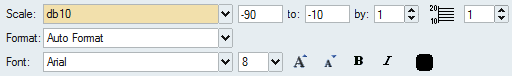
On the Y-axis block, right-click. In the floating panel
that appears, from the Scale drop down list, select
db10.
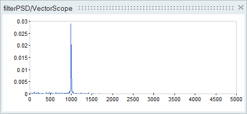
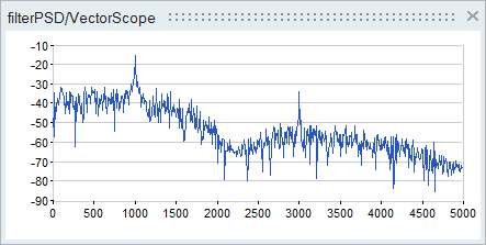
The power spectrum density graph appears as you see in the following figure.
Two peaks at frequencies are present: 1000Hz and 3000Hz. The 3000Hz peak is
lower because the original signal is attenuated by the Chebychev low-pass
filter.
Downsample the Output of the Buffer
Reduce the sampling frequency of the buffer.
From the Palette Browser > Activate > ActivationOperations, drag 1 ReSampleClock block into the
diagram.
Both activation input ports of the Buffer block are triggered by the
SampleClock block at 10,000Hz. This trigger forces the blocks downstream,
including the FFT and VectorScope blocks, to run at 10,000Hz which can result in
unnecessary computation and scope generation. The addition of the ReSampleClock
block ensures that the Buffer block updates the output only when
required.
Assemble and connect the blocks like this:
On the ReSampleClock block, double-click. From the block
dialog that appears, for Down Sampling Factor, enter
N.
Changing this parameter ensures the outgoing activation is triggered
whenever N points are sampled by the Buffer block when
full.
On the ribbon, select Run.
Running the simulation takes less time to finish than in the previous
iteration, though the results are similar:
 , then Save Model
 .
.
 .
.
 Note: The one-sided power spectral density is computed with the equation P= 2 ∗ |ff | ^ 2/(F∗N)
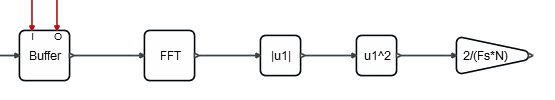
 .
.