Inbuilt Material Properties
Fluid Properties
- Air as a perfect gas
- Mixture of air as a perfect gas and steam
- Mixture of air as a perfect gas and real gas
- Mixture of two real gases
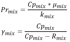
- γ
- Specific heat ratio
- Cp
- Specific heat at constant pressure
- R
- Gas constant
- K
- Thermal conductivity
- μ
- Viscosity
- Pr
- Prandtl number
- Nomenclature
- T
- Fluid temperature
- Ru
- Universal gas constant
- X
- Secondary fluid mass fraction in pounds of second fluid per pound of mixture.
- MW1
- Molecular weight of fluid 1
- MW2
- Molecular weight of fluid 2
Air Properties
Ideal Gas Assumption
If air is assumed to behave as an ideal gas, its properties are determined by functions dependent on temperature only. The specific heat ratio, taken from NACA 1135, equation 180, is given as:
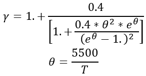
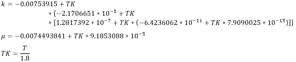
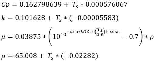
Thermal conductivity and viscosity are assumed to follow Sutherland’s Law. The following equations, taken from White, are used:
Using a value for the molecular weight of air of 28.96451, the gas constant becomes:
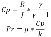
The specific heat and Prandtl number for air are then calculated from the above using the equations:
The range of validity of these air properties is –300 F to 3500 F.
Steam Properties
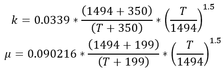
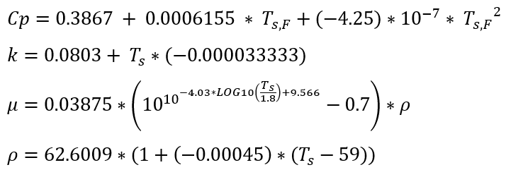
The steam properties were derived from ASME steam tables. The thermodynamic properties cover the range where the fluid is a vapor for temperatures between 100 ℉ and 1500 ℉ and pressures between 1.0 psia and 1500 psia. Specific heat ratio and the inverse of specific heat at constant pressure are contained in table form in the program, and linear interpolation by temperature and pressure is used to extract values. The transport properties k and μ are functions of temperature only and are calculated using the equations:
The saturation temperature of steam is contained in tabular form and is checked to ensure that chamber temperature remains in the superheated range in all chambers. The solution is stopped if this error occurs. A warning is displayed and/or printed if the temperature in a chamber gets within 50 ℉ of saturation.
Properties of Mixed Air, Steam, and Real Gases
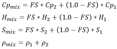
Flow Simulator has the capability to analyze systems with mixtures of steam, air, and real gases (for example, methane and carbon dioxide). The system used to do this is approximate because ideal gas assumptions employ Cp rather than enthalpy for the calculation of the temperature of mixing streams of different fluids.
The mass weighted mixing model is always used for the thermodynamic properties of specific heat at constant pressure. The partial pressure of the fluid is used to obtain properties for steam and real gas. Ideal air properties are not a function of pressure. The mass weighted mixing equations, presented here for specific heat, entropy, enthalpy, and density, are as follows:
The molecular weight and gas constant of the mixture are calculated using:
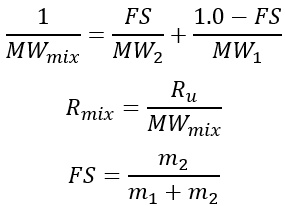
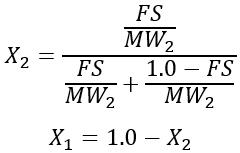
The viscosity and conductivity of the mixture are calculated using molecular mixing models. For the molecular mixing model, the mole fraction of the second fluid, X2, is calculated from the second fluid mass fraction as:
Specific equations for the transport properties were obtained from reference [6].
Viscosity for the air-steam mixtures (and viscosity and thermal conductivity for mixtures with real gas) are calculated using the Chapman-Enskog Kinetic Theory from the equation:

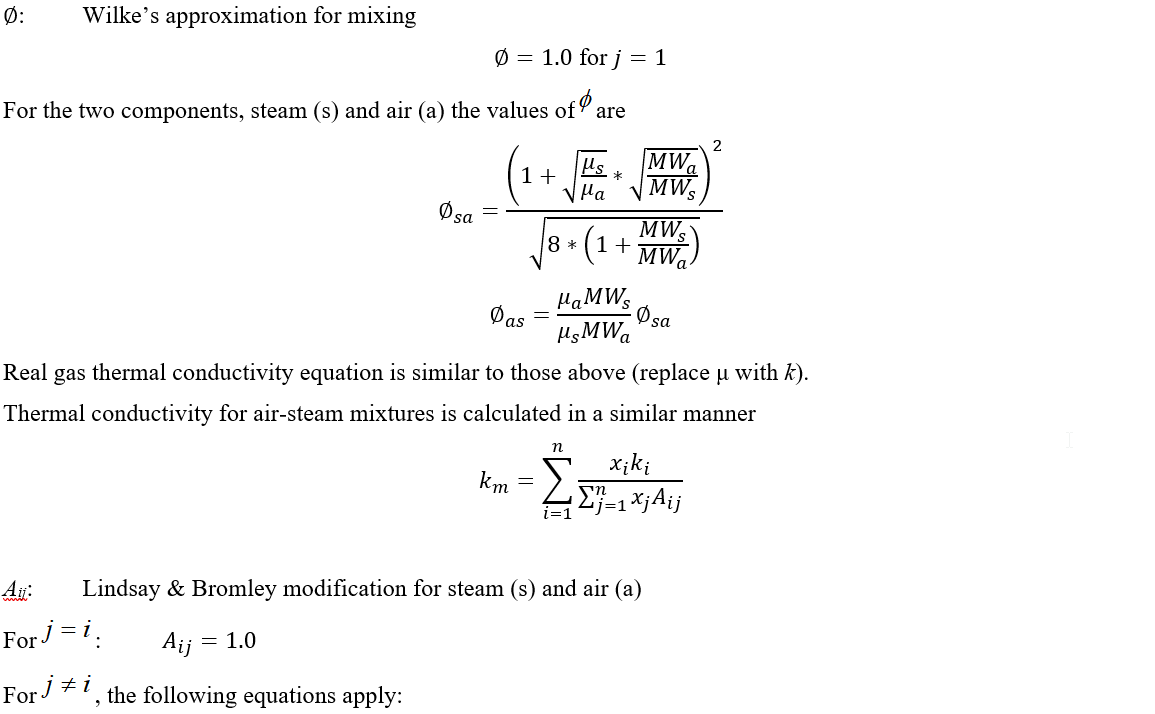
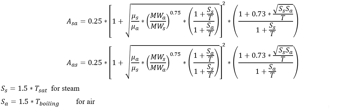
All temperatures are in absolute units.
The Prandtl number and the specific heat ratio for the mixture are computed using the mixed properties:
Incompressible Liquid Properties
- Water
- Jet A
- Mil PRF 23699 oil
- Mil 7808 oil
- VG-32 oil
- Ethylene glycol - water solution
- Propylene glycol - water solution
- T
- Temperature of the solution in Celsius
- x
- Mass fraction of Ethylene Glycol
Density Calculation - D. Bohne, S. Fischer, and E. Obermeie: Thermal Conductivity, Density, Viscosity, and Prandtl-Numbers of Ethylene Glycol-Water Mixtures
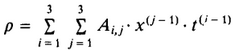
Figure 1.
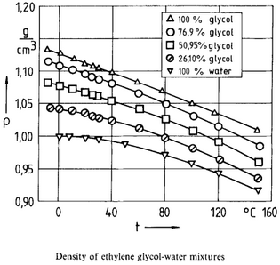
Figure 2.
Thermal Conductivity Calculation: D. Bohne, S. Fischer, and E. Obermeie: Thermal Conductivity, Density, Viscosity, and Prandtl-Numbers of Ethylene Glycol-Water Mixtures
κH20 = 0.570990 + 1.67156e-3 * T - 6.09054e-6 * T2
κEG = 0.245110 + 1.75500e-4 * T - 8.52000e-7 * T2
κCONST = 0.6635 – 0.3698 * x – 8.85e-4 * T
κSOL = (1-x) * kH20+ x * κEG - κCONST * (κH20- κEG ) * (1-x) * x
κSOL = κSOL * 0.5781759824 (convert from W/m-K to BTU/hr-ft-degR)
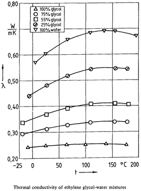
Figure 3.
Dynamic Viscosity Calculation: Tongfan Sun and Amyn S. Teja: Density, Viscosity, and Thermal Conductivity of Aqueous Ethylene, Diethylene, and Triethylene Glycol Mixtures between 290 K and 450 K
µEG = -3.613590 + 986.5190 / (T + 127.8610)
µH20 = -3.758023 + 590.9808 / (T + 137.2645)
µCONST = -0.165301 -0.287325 * x +1.10978e-3 * T
µSOL = EXP [ x * µEG + (1-x) * µH20 + (µEG - µH20)* x * (1-x) * µCONST]
µSOL = µSOL * 2.4190883293091 (convert from mPa/s to lbm/hr-ft)
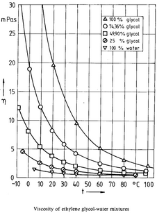
Figure 4.
Specific Heat Calculations/Property Tables (source: Engineering Toolbox (https://www.engineeringtoolbox.com/)
Propylene Glycol - Water Solution, Tongfan Sun and Amyn S. Teja: Density, Viscosity and Thermal Conductivity of Aqueous Solutions of Propylene Glycol, Dipropylene Glycol, and Tripropylene Glycol between 290 K and 460 K
- T
- Temperature of the solution in Celsius
- w
- Mass fraction of ethylene glycol
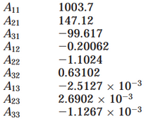
Figure 5. Density Calculation
Thermal conductivity calculation:
µH20 = 0.570990 + 1.67156e-3 * T - 6.09054e-6 * (T2)
µPG = 0.191160 + 1.19999e-4 / (T + 9.24590e-7)
µCONST = 0.362200 + 9.03450e-2 * FS - 2.0935e-4 * T *
µSOL = (1-FS) * µH20 + w * µPG - µCONST * (µH20 - µPG) * (1-w) * w
µSOL = µSOL * 0.5781759824 (convert from W/m-K to BTU/hr-ft-degR)
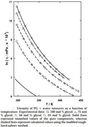
Figure 6.
Specific Heat Calculations/property tables - source is Engineering Toolbox (https://www.engineeringtoolbox.com/)
Dynamic Viscosity Calculations/property tables - source is Engineering Toolbox (https://www.engineeringtoolbox.com/)
VG 32 Oil
 Figure 7. Density(Lbm/ft3) for VG32 Oil
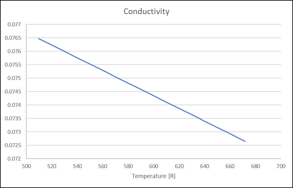 Figure 8. Thermal Conductivity (Lbm/hr.ft.F) for VG32 Oil
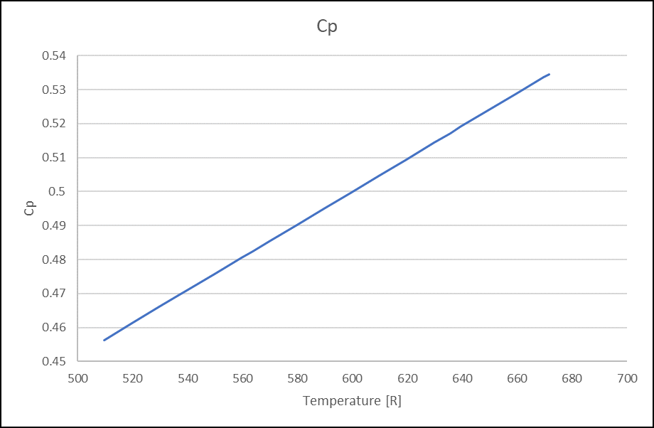 Figure 9. Specific Heat (Btu/Lbm.degR) for VG32 Oil
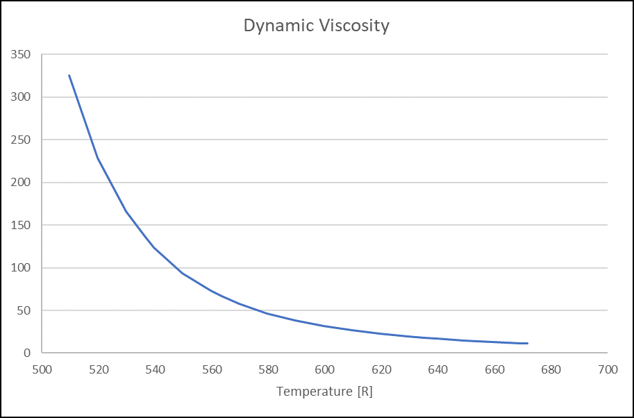 Figure 10. Dynamic Viscosity(Lbm/hr.ft) for VG32 Oil
Water
Water properties are implemented as tables in Flow Simulator. The tables for each fluid property are plotted below:
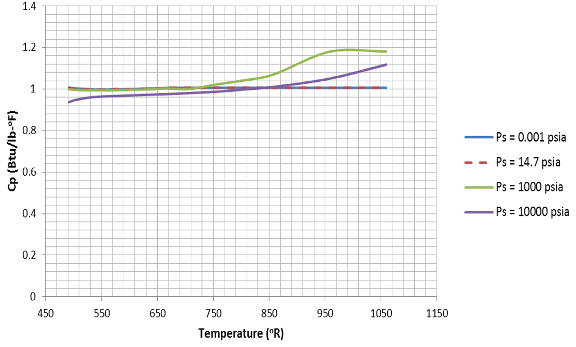 Figure 11.
 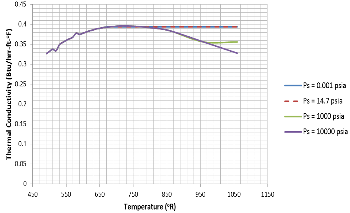 Figure 12.
 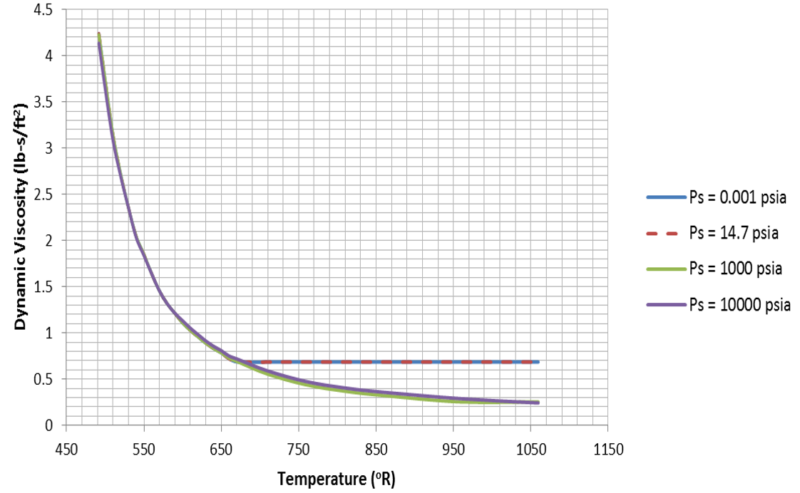 Figure 13.
 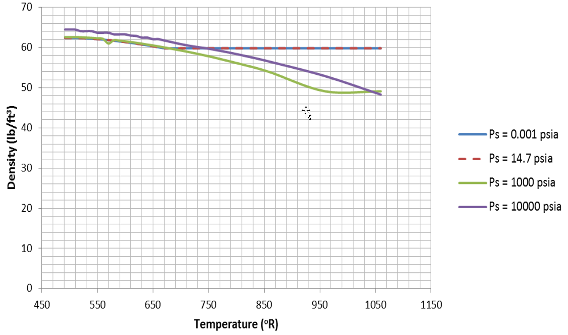 Figure 14.
 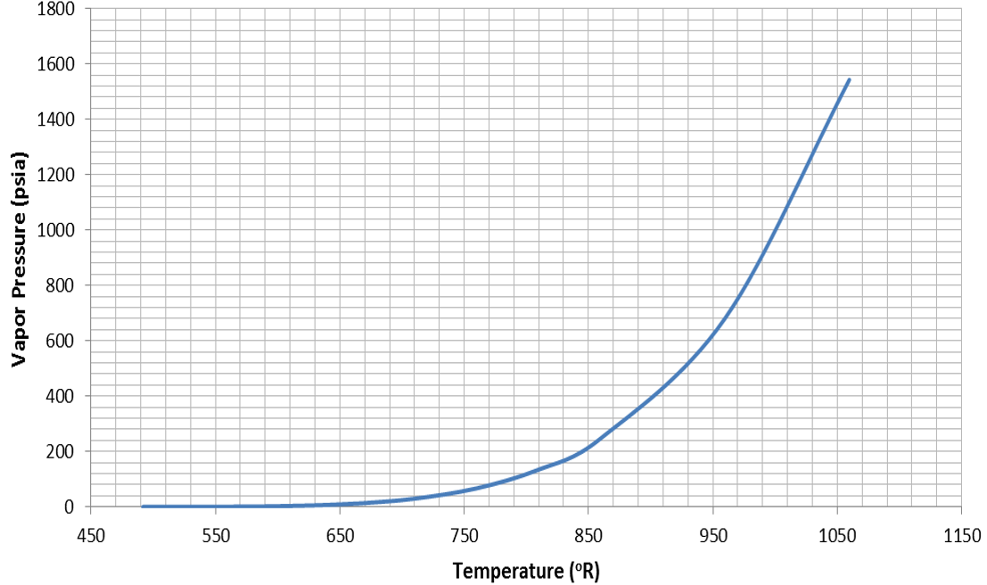 Figure 15. Vapor Pressure for Water
Solid Material Properties
- Stainless Steel 321
- Inco 625
- SuperWool 607
- Ceramic Paper
- PTFE_PBI
- Stainless Steel 321
- ρ = 501.11 ! lbm/ft^3
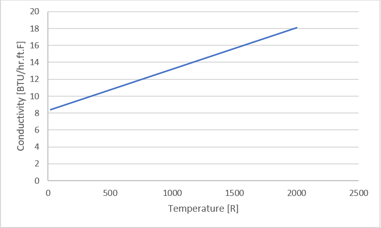 Figure 16.
 - Inco 625
- ρ = 523.58 ! lbm/ft^3
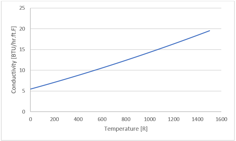 Figure 17.
 - Superwool 607
- ρ = 13.10988 ! lbm/ft^3
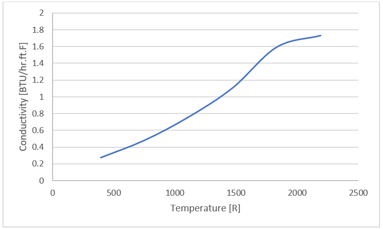 Figure 18.
 - PTFE_PBI
- k = 1.733368 ! BTU/hr.ft.F