Parametric distribution in Flux
Introduction
- The number of cores (i.e the number of running Flux in parallel);
- Principles;
- How to set up a parametric distribution with Windows OS on a single machine;
- How to set up a parametric distribution with Linux OS on a single machine;
- Define a parametrized scenario in Flux
- Example of application.
Principles
The parametric distribution allows the user to save computation time by parallelizing several independent configurations of a finite element problem with different values of I/O or geometric parameters varying in the scenario instead of running them sequentially. To set-up a distributed computation, a Flux master project is mandatory in order to compute all its sub-projects having an independent configuration.

Figure 1. Picture illustrating a parametric distribution, a Flux master is controlling several Flux Slaves with independent configurations of geometric or I/O parameters.
- They all ran with only one core;
- The amount of memory assigned to the Flux Slaves is set to the same value as the Flux Master, if the memory is setted to Dynamic for the Flux Master, the Flux Slaves will also start with dynamic memory.
How to set up a parametric distribution with Windows OS on a single machine
In Flux 2D and in Flux 3D, the parametric distribution options (number of Flux Slaves in parallel) may be setted in the Supervisor's options or by clicking on the button Distribution manager in the bottom right of the Supervisor. For the Flux Skew module, this feature is not yet available and will run automatically in sequential mode.
In any case, the parametric distribution may be setted as follows:
- The Distribution manager may be started in the Supervisor's options,
in the Parallel Computing menu, in the section Distributed
Computing and then Parametric Distribution click on the
button Set local ressources as shown below;
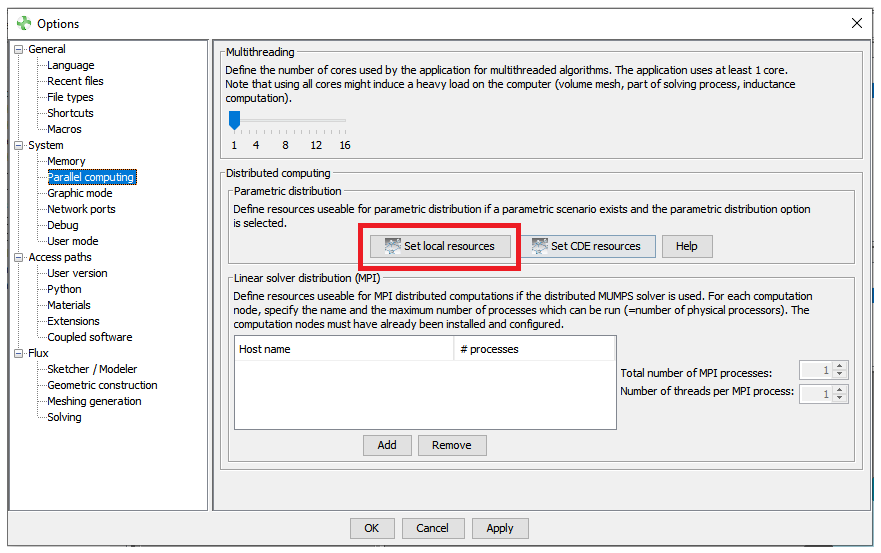
Figure 2. The supervisor's options allowing the user to set the parametric distribution. - An additional window Distribution manager should appears and is asking to allow some resources (Number of Flux Slaves in parallel) for the parametric distribution, click on Allow;
- The Distribution manager then asks for the Number of concurrent
Flux as follows:
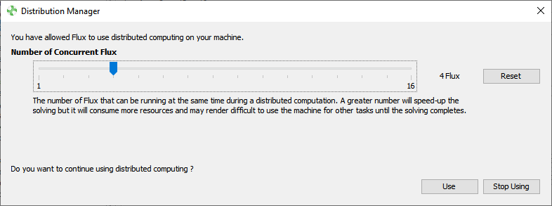
Figure 3. The distribution manager asking for the Number of Concurrent Flux.Note: This number is directy linked to the number of cores available on the machine, the numbers of varying parameters are automatically distributed over the number of concurrent Flux. - Finally, click on Use to complete the parametric distribution
How to set up a parametric distribution with Linux OS on a single machine
In Flux 2D and in Flux 3D, the parametric distribution options (number of Flux Slaves in parallel) may be setted in the Supervisor's options or by clicking on the button Distribution manager in the bottom right of the Supervisor. For the Flux Skew module, this feature is not yet available and will run automatically in sequential mode.
In any case, the parametric distribution may be setted as follows:
- The parametric distribution may be started by clicking the button
Distribution manager in the bottom right of the Supervisor as
shown below.

CAUTION:In Windows OS this button will start the CDE distribution toolFigure 4. The distribution manager button in the Flux Supervisor. .
. - An additional window Distribution manager should appears and is asking to allow some resources (Number of Flux Slaves in parallel) for the parametric distribution, click on Allow;
- The Distribution manager then asks for the Number of concurrent
Flux as follows:

Figure 5. The distribution manager asking for the Number of Concurrent Flux.Note: This number is directy linked to the number of cores available on the machine, the numbers of varying parameters are automatically distributed over the number of concurrent Flux. - Finally, click on Use to complete the parametric distribution
- The Distribution manager may also be started in the Supervisor's options, in the Parallel Computing menu, in the section Distributed Computing and then Parametric Distribution click on the button Set local ressources;
Define a parametrized scenario in Flux
- Check the box Parametric distribution in the selected
Scenario.Note: All the varying parameters should be declared as Controlled parameters in the Control parameters tab of the scenario as depicted below in Figure 6.

Figure 6. Scenario GUI box, highlightning in (1) the Parametric distribution that is enabled and in (2) a list a of several varying parameters.
Example of application

Figure 7. Three-phase, eight-pole permanent magnet synchronous machine (PMSM) described in Flux 2D.
- The speed which is declared as an I/O parameter controlled by the scenario and that is used by the rotating mechanical set
- The shape of the magnet with the magnet outer arc value α setted with
a geometrical parameter as depicted below.

Figure 8. Magnet outer arc parametrized with a geometrical parameter that may be selected as a varying parameter during the scenario.
| Magnet outer arc α (degrees) | Speed (rpm) | |
|---|---|---|
| Minimum value | 130 | 1300 |
| Maximum value | 170 | 1700 |
| Step value | 10 | 100 |

Figure 9. Graph representing the time computation evolution in function of the number of concurrent Flux.