Block Category: Matrix Operation
Input: If the input to the fft block is not an integral power of 2, automatic zero padding is performed to make the input vector size an integral power of 2. This is a standard procedure in FFT computation. The output of the fft block is the complex Fourier coefficients vector, where each adjacent pair of elements are the real and complex parts beginning with the first element, which is the first real value. For example, an fft output = [1 2 3 4 5 6] is interpreted as the having three output coefficient values: 1+j2, 3+j4, and 5+j6. The real and imaginary elements can be separated into two vectors using the reshape block. Applying the fft output to a reshape block with dim1 = 2 and dim2 = 3 produces a matrix with 2 rows and 3 columns, where row 1 are the real elements and row 2 are the imaginary elements: [1 3 5; 2 4 6].
Description: The fft block converts data from time domain to frequency domain computing an n-sample FFT at every simulation time step, where n is the length of the input vector.
Label: Indicates a user-defined block label that appears when View > Block Labels is activated.
1. Computation of FFT and inverse FFT
Consider a simple example, where a sinusoidal signal is converted to frequency domain via FFT, and then reconstructed using inverse FFT.
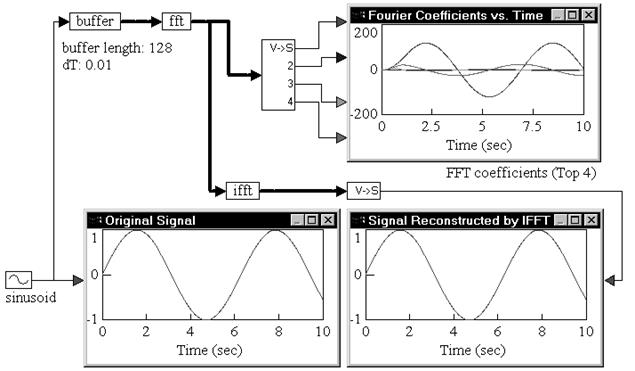
A sinusoid block generates a sinusoid signal with a frequency of 1 rad/sec. The signal is passed through a buffer block of length 128 samples and a dT of 0.01. The output of the buffer block is connected to an fft block, which computes a 128-sample FFT of the original sinusoid at a sampling rate of 0.01.
The output of the fft block is Fourier coefficients. The individual coefficients are accessed using a vecToScalar block. The first four coefficients are plotted to show their variation with time.
Signal reconstruction is performed by feeding the output of the fft block to an ifft block to compute the inverse FFT. The output of the ifft block is a vector of length 128 samples. The contents of this vector are just 128 sinusoid reconstructions, with each sinusoid trailing the preceding sinusoid by an amount equal to the sampling rate.
The first element in the ifft output vector does not have any delay because zero time has elapsed between the FFT and inverse FFT phases. In most real-world situations, however, there is a small, non-zero delay between the input signal and its reconstruction that is introduced by the processor performing the numerical computations of FFT and inverse FFT algorithms.
2. Computation of FFT with 100Hz sampling frequency and 128 sampling points
In this example, each point in the FFT output array has a frequency resolution calculated as:
del_freq = Sampling_frequncy/No. of sampling points = 0.78125 Hz
The input signal has a frequency of freq_resoultion *2 = 1.5625 Hz and an offset of value 2.
In the FFT output, you see peaks only at point0 (dc offset) and point2 ( freq = 1.5625 Hz) highlighted in yellow.
