Actual Point Count: Displays the number of data points plotted.
Clear Overplot Y: Clears all signal traces from a plot.
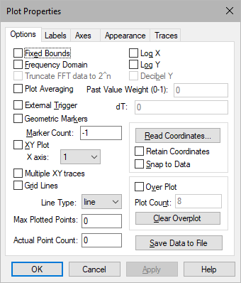
Decibel Y: Rescales the y-axis to display the values in decibels.
dT: When you activate External Trigger, the plot block acquires data at an unknown rate. dT allows you to specify the delta time between data points.
External Trigger: Determines whether simulation data is displayed in the plot based on the value of an external trigger. When activated, a round input connector is attached to the plot block. When signal values entering the external trigger are 1, simulation data is plotted; when signal values entering the external trigger are 0, simulation data is not plotted. This parameter is particularly useful when plotting vector data. See Plotting vector data. To save vector data to a file and read it in another application, such as Excel, use the export block.
Fixed Bounds: Specifies the region of the plot you want to view. Note that the plot will always plot from the Start to the End values in the System Properties dialog box. When you activate XY Plot, the Y Upper Bound and Y Lower Bound values under the Axes tab are used.
Frequency Domain: Obtains the frequency power spectrum using the Fast Fourier Transform (FFT) algorithm.
Do not obtain frequency power spectrum data until after you have run a simulation. If you halt the simulation prematurely, the fidelity of the FFT is diminished.
If your frequency domain plot produces unexpected peaks, check the simulation step size to verify that your sampling rate is adequate for obtaining accurate results. Then, based on the simulation step size and range, check Plotted Points to verify that you are indeed plotting each time step.
Geometric Markers: Overlays signal traces with geometric markers.
Grid Lines: Extends grid lines from the vertical and horizontal axis coordinates. The vertical and horizontal spacing of grid lines is controlled by the spacing of the axis coordinates. Embed automatically establishes reasonable axis coordinate spacing and hence controls the grid frequency.
Line Type: Point displays signal values as individual data points. Point plots show the separation of data as time advances.
Line connects data points with solid line segments. On color displays, line segments are the color of the corresponding input connector tab. On monochrome displays and printers, line patterns distinguish signal traces. You may have to lower the point count to allow enough room between data points for the pattern to be displayed. If this is not satisfactory, you can overlay signal traces with geometric markers.
Discrete holds the Y value constant from point to point. A discrete plot is helpful when data points are irregularly spaced and you don’t know where the curve is accurate.
Log X and Log Y: Allow data to be plotted in logarithmic and semi-logarithmic coordinate systems. When you specify a logarithmic or semi-logarithmic plot, you cannot plot negative values on the log axis. Any negative value will be clipped to the low end of the scale. When neither parameter is activated, the plot defaults to linear.
Marker Count: Determines the number of markers overlaid on each signal trace. By default, Embed overlays each data point in a signal trace with a marker; however, if this is not satisfactory, you can enter a new number in Marker Count. Entering -1 in this box indicates all data points have markers associated with them.
Max Plotted Points: Determines the smoothness and accuracy of a plot. The more data points you plot, the smoother and more accurate the plot. However, increasing the number of plotted data points also increases the time it takes to print and display the plot.
The maximum number of data points that can be plotted is 250 million. Entering 0 plots every data point.
If you know the maximum number of data points you want plotted in all your plots, you can set it as the default.
Multiple XY Traces: Creates two independent XY plots, which allows two signals to be superimposed. The XY Plot parameter must be activated to use Multiple XY Traces.
Over Plot: Displays the results of multiple simulation runs in a single plot. This allows for better insight into how small changes can affect overall system performance. Enter the number of overplots in Plot Count.
Past Weight Value: Specifies the values of the previous simulation runs to be averaged into the current run. Specify the value as a fraction of 1.
Plot Averaging: In multi-run simulations, the values of the previous run are averaged into the current run using Past Value Weight as a fraction of 1. This is useful for filtering out noise.
It is recommended you activate Fixed Bounds. In addition, you must activate Auto-Restart under System > System Properties > Range.
Plot Count: Sets the number of overlapping plots.
Read Coordinates: Overlays the plot with a set of crosshairs and displays crosshair position at the bottom of the plot. When you click the mouse button, Embed freezes the crosshairs. Click again to erase the crosshairs.
Retain Coordinates: Displays two crosshairs. One crosshair is frozen at the last known x,y position. The other is controlled by the position of the pointer.
Save Data To File: Opens the Select File dialog box to specify a file to which the plot data is to be saved.
Snap To Data: Causes the data point closest to the pointer to have a magnetic-like pull on the crosshair. As you move the pointer, the crosshair continues to jump to the closest data point.
Truncate FFT Data to 2^n: Truncates data down to the nearest power of 2. If you do not activate this parameter, the data buffer is padded with zeros to round up to the nearest power of 2. This parameter can be turned on only when Frequency Domain is activated.
XY Plot and X Axis: Together, XY Plot and X Axis let you use one input signal to represent X coordinate generation. As time advances, the remaining input signals are plotted relative to the x-axis signal.