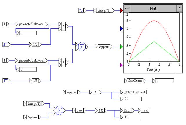
To solve a constrained optimization problem, you use globalConstraint blocks. These blocks identify constraints that depend on parameterUnknowns and are more complicated than the bound constraints.
To illustrate the use of the globalConstraint block, the previous problem can be modified by constraining the area under the approximating function so that it cannot exceed 0.4.
To modify CURV2P
1. Add the following blocks to the diagram:
•Under Block > Optimization, add a globalConstraint block
•Under Blocks > Integration, add an integrator block
•Under Blocks > Signal Consumer, add a display block
2. Make a copy of the Approx block.
3. Wire the output of the Approx block into the integrator block.
4. Wire the output of the integrator block into the globalConstraint and display blocks.
The upper and lower bounds for the globalConstraint block are established in its dialog box. You only have to assign these values once; after that, the upper and lower bounds are remembered.
To set the upper and lower bounds
1. Right-click the globalConstraint block.
2. Make the following selections in the dialog box:
a. In the Upper Bound box, enter 0.4.
b. In the Lower Bound box, enter 0.0.
c. Click OK, or press ENTER.
The optimization parameters set in the previous example are valid for this example. If you skipped the previous example, you must set them now.
To set the optimization parameters
1. Choose System > Optimization Properties.
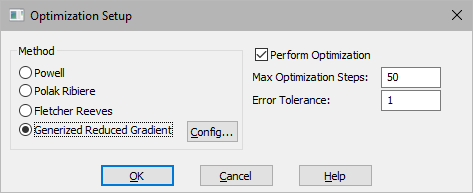
2. Make the following selections:
•Under Method, select Generalized Reduced Gradient to perform constrained optimization.
•Activate Perform Optimization.
•In Max Optimization Steps, enter 100 to set the limit on the number of optimization steps.
•In Error Tolerance, enter 0.0001. This parameter defines the relative accuracy of the simulation runs. In this case, three digits of accuracy are found in the solution.
3. Click OK, or press ENTER.
To solve the constrained optimization problem, click on the
 toolbar button.
This constrained optimization run yields the parameterUnknown values of 1.73 and 1.85 and the cost value of 6.21e-2. The constraint is at its upper bound of 0.4 as should be expected.
Note: The exact answer to the analytic problem posed here may differ from the computed answer. This discrepancy shows up because the integration methods are not exact. You can verify this by decreasing the integration step size in the System > System Properties dialog box and rerunning the simulation. The Embed solution to this problem differs (due to numerical truncation errors) from the analytic solution. Taking smaller step sizes makes this relationship clear.