
This example uses the CURV2P diagram, which represents a simple two-parameter curve fitting application involving the approximation of the function Sin (πt) in the interval from 0 to 1. You will approximate this function by another function composed of two straight line segments. There are no constraints in this problem.
Diagram Location: Examples > Optimize
Diagram Name: CURV2P
When you open CURV2P, the following diagram appears on the screen:
The function Sin (πt) is produced by a sinusoid block with frequency π and amplitude 1. It is wired into a variable block labeled Sin ( pi*t ). The approximating function is produced with two step blocks and two integrator blocks. This function is wired into a variable block labeled Approx. Both curves are plotted.
The cost or objective function is computed by integrating the squared difference of the two curves, (Sin ( pi*t ) - Approx)2 , from 0 to 1. The error is wired into a cost block to identify it as the objective function.
Each of the parameterUnknowns is wired to a const block with value 1. This provides starting values for the parameterUnknowns or decision variables. A simulation run plots the two curves and computes the error for the starting values as 0.178.
To find the best multipliers for the approximating function to produce the smallest error, the multipliers are wired to parameterUnknown blocks (which alert Embed that optimization may be performed on these decision variables) and then into a display block so that the parameters can be monitored during the optimization run. Upper and lower bounds of 10 and -10 have been set for these parameters in the parameterUnknown blocks. To view or change the bounds, right-click the parameterUnknown block.
To solve the optimization problem, you use the Optimization Properties command. Optimization Properties lets you select constrained optimization.
To set the optimization parameters
1. Choose System > Optimization Properties.
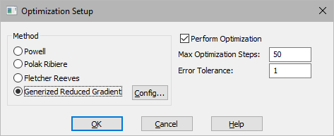
2. Make the following selections:
•Under Method, activate Generalized Reduced Gradient. When you activate this parameter, constrained optimization is used.
•Activate Perform Optimization.
•In Max Optimization Steps, enter 100. Sets a limit on the number of optimization steps.
•In Error Tolerance, enter 0.0001. This parameter defines the relative accuracy of the simulation runs. In this case, three digits of accuracy are found in the solution.
3. Click OK, or press ENTER.
To solve the problem
•From the Toolbar, click on the  toolbar button to start the
optimization.
toolbar button to start the
optimization.
Observe the following after 28 simulation runs (reference $runCount in the diagram):
•The cost block has changed from 0.178 to 5.82e-3
•The parameterUnknown block (upper part of the diagram) has changed to 2.38
•The parameterUnknown block (lower part of the diagram) has changed to 2.29
In addition, a report is written to VSMGRG2.TXT that provides more information on the optimization process.