Isovalues: about

Plotting of isovalues

Spatial scalar quantities can be displayed with color shaded isovalues on different supports.

For spatial vectorial quantities the modulus as well as the components can be displayed with isovalues.

Support

The support for the plotting of isovalues is always a surfacic support. In Flux PEEC, the supports available are:

external surfaces of unidirectional conductors
external surfaces of bidirectional conductors
2D grids

Computation algorithm

The computation of isovalues is done in two steps:

first, the spatial quantity considered is calculated at some relevant points of the support surfaces; these points depend on the physical quantity considered, but in general they are highly linked to:

for unidirectional conductors, to the mesh and the additional points due to the discretization in the length for the post processing *
for bidirectional conductors, to the mesh
for 2D grids, to their own discretization as described in § 2D grids: about

then, an interpolation algorithm makes it possible to compute the quantity considered at intermediate points enabling the smoothing of the isovalues

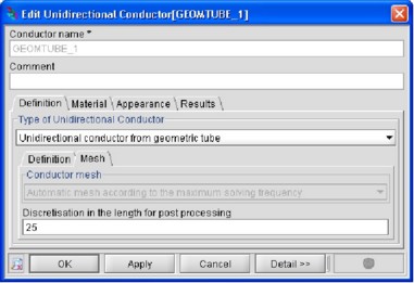
Note: * To discretize in the length a unidirectional conductor, the user must first create it and then edit its features from the Data tree . In the Mesh tab of the window which appears, the user can define the number of discretization points along the length, as shown in the figure below.

Spatial quantities

The spatial quantities that can be displayed with isovalues are:

the modulus and the three components (X, Y and Z) of the current density
the Joule losses density
the modulus and the three components (X, Y and Z) of the magnetic flux density
the modulus and the three components (X, Y and Z) of the Laplace force density: the average component or the 2ω pulsating component