Extractor Definitions
Import an .stl file and use it as a sampling surface for variable fields. This surface can be visualized during post-processing and can enable various advanced post-processing. The feature supporting this ability is called an extractor.
Extractors are intended to provide more flexible postprocessing and interpolation options by enabling runtime interpolation, access to solid data, moving interpolation surfaces, custom output times and providing variables that are not immediately available through regular field output.
An extractor consists of a set of interpolation points that may follow a solid phase of interest and interpolate different simulation variables at set sampling intervals. Similar to probes and phaseinfo, extractors have access to all simulation data of each phase, solid or fluid, at all times and thus can produce more accurate interpolations, instantaneous or periodically time averaged, compared to those solely relying on field output.
An .stl file is used to define an extractor surface. This surface may match a solid surface or lie completely within the flow. The .stl file must be in binary format and have correct facet normals. Multi solid .stl files will be treated as a single solid, skipping attributes field, as only one surface per extractor is allowed.
Facet centers will be used as interpolation points. All extractor results are written into EXTRACT directory under case data directory. Each extractor generates a series of VTK polydata (vtp) files under a directory with the same name as the extractor itself as well as a pvd file directly under EXTRACT directory. Extractors may have two types of output:
- Unsynchronized (unsync): the outputs are written according to the internal output interval of the extractor and do not necessarily coincide with the field output write times. The output interval is a constant value. This extractor output may not be suitable for visualization in the same postprocessing session as field outputs.
- Synchronized (sync): in addition to unsync outputs, extractor outputs may also be written at field output write times. Field output time internals may be variable or constant. These outputs are suitable for visualization alongside field outputs.
The solver creates a VTK multiblock (vtm) file per filed output time under sync_output directory when sync output is activated for at least one extractor. This vtm file references relevant vtp files of each extractor requesting a sync output. Additionally, a sync_output.pvd file referencing the vtm files is created and placed directly under EXTRACT. The goal is to facilitate the loading of sync output in the same postprocessing session as the field data. You may match sync and unsync extractor output times when field output intervals are constant. Figure 1 provides a sample directory structure of the EXTRACT directory. The extractor directory and pvd file names are replaced with the names specified in the cfg file definition of the extractor.
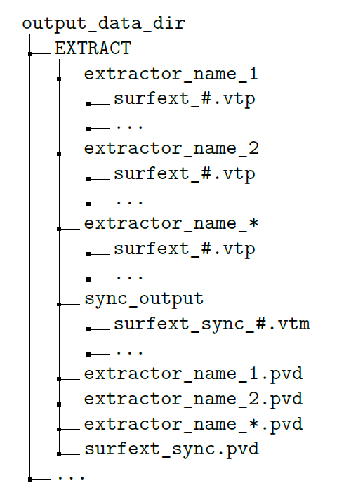
Figure 1. Directory Structure of Extractor Output under EXTRACT Directory
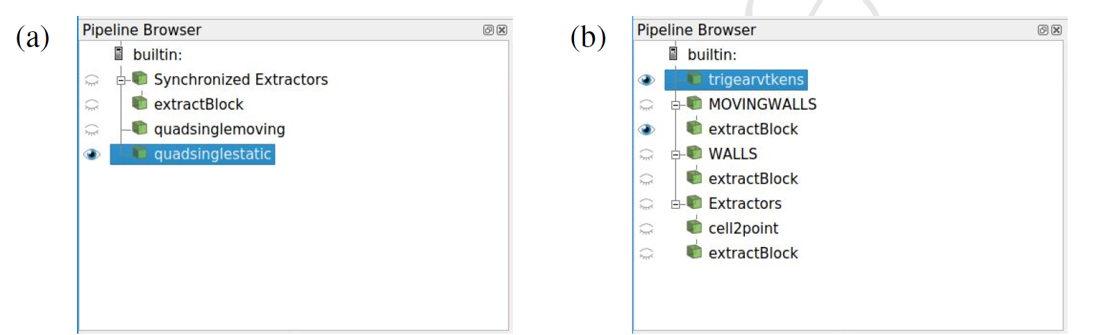
Figure 2. Pipelines of Sample State Files Loaded in ParaView 5.9.1. (a) extractor.py; (b) PostJobName.py
- Fluid velocity
- Fluid velocity in the direction of surface normal (normal velocity)
- Fluid velocity on the surface (parallel velocity)
- Fluid pressure
- Fluid density
- Kernel volume integral over all resolved phases (Shepard Summation in ParaView with both fluids and solids)
- Kernel volume integral over all fluid phases (Shepard Summation in ParaView with only fluids)
- Sampled particle count over all phases
- Sampled particle count over all fluid phases
- Volume fraction of each fluid phase over all phases
- Volume fraction of each fluid phase over all fluid phases
- Cumulative fluid contact time for each fluid phase
- Cumulative time normalized fluid contact time for each fluid phase
- Periodically time normalized fluid contact time for each fluid phase
Some of the abbreviations used as the requested output suffixes are as follows:
- oap - over all phases
- ofp - over fluid phases
- pta - periodically time averaged
Periodically time averaged values do not extend over different legs of a run. For example, time averaging restarts at a new leg of a simulation. Fluid contact time variants of cumulative and cumulative time normalized are based on continuous summation during the current leg of the simulation. They are only reset at the beginning of a new leg of the run. This means at the beginning of a clean or recon run, cumulative and cumulative time normalized fluid contact times start from zero.
To simplify the loading and viewing process of extractor outputs in ParaView, nanoFluidX writes an additional python state file, extractor.py, under PVSTATE directory. This state file includes both sync and unsync outputs. Sync output pipeline includes an additional extractBlock (Extract Block) filter to select the visible extractors. Other state files with field data (particles.py from nanoFluidX and PostJobName.py from nanoFluidX[c]) have been updated to include extractor sync output with cell2point (Cell Data to Point Data) and extractBlock filters. When loaded individually in ParaView, the sync output pvd file surfext_sync.pvd will appear as a multiblock data file and an Extract Block filter is required to select an individual extractor or a group of extractors. The extractors write their data on face centers (cell data in VTK/ParaView terminology) and this data is considered to be constant across the cell in ParaView. Using a Cell Data to Point Data filter produces a continuously varying representation. Sample pipelines are shown in Figure 2. The archive created by nFX[c] now includes EXTRACT directory and extractor.py state file for easier movement of data for postprocessing.
Extractors may have a noticeable footprint on simulation time depending on the number of samples and frequency of unsync outputs. It is recommended to use an extractor output time interval larger than phaseinfo output time and shorter than or equal to field output time to balance computational cost and quality of the extractor output. The number of samples depends on the unsync output interval length and the nature of the problem being simulated.
extractors
{
    extractor
    {
        extractor_name                            surfextname
        extractor_stlfile                         surfext.stl
        extractor_dtoutput                        1.0
        extractor_nsample                         20
        extractor_motphs                          -1
        extractor_syncoutput                      false
        extractor_output_rho_i                    false
        extractor_output_press_i                  false
        extractor_output_vel_i                    false
        extractor_output_velnrm_i                 false
        extractor_output_velpar_i                 false
        extractor_output_kervolint_oap_i          false
        extractor_output_kervolint_ofp_i          false
        extractor_output_prtlcount_oap_i          false
        extractor_output_prtlcount_ofp_i          false
        extractor_output_volfrac_oap_i            false
        extractor_output_volfrac_ofp_i            false
        extractor_output_rho_pta                  true
        extractor_output_press_pta                true
        extractor_output_vel_pta                  true
        extractor_output_velnrm_pta               false
        extractor_output_velpar_pta               false
        extractor_output_kervolint_oap_pta        true
        extractor_output_kervolint_ofp_pta        true
        extractor_output_prtlcount_oap_pta        false
        extractor_output_prtlcount_ofp_pta        false
        extractor_output_volfrac_oap_pta          false
        extractor_output_volfrac_ofp_pta          false
        extractor_output_fct_ptn                  true
        extractor_output_fct_ctn                  true
        extractor_output_fct_c                    true

        extractor_htc_nrpee_bulktemp              273.5
        extractor_output_htc_nrpee_i              false
        extractor_outputtxt_htc_nrpee_i           false
        extractor_output_htc_nrpee_pta            false
        extractor_outputtxt_htc_nrpee_pta         false

        extractor_output_htc_emp_i                false
        extractor_outputtxt_htc_emp_i             false
        extractor_output_htc_emp_pta              false
        extractor_outputtxt_htc_emp_pta           false
    }
}- extractor_name
- Name of the surface extractor.
- extractor_stlfile
- Name of the stl file used for defining the interpolation points of surface extractor.
- extractor_dtoutput
- Time interval between non-synchronized outputs, starting from beginning of this run segment.
- extractor_nsample
- Time interval between non-synchronized outputs, starting from beginning of this run segment.
- extractor_motphs
- PhaseID of the MOVINGWALL phase which surface extractor is to follow.
- extractor_syncoutput
- Additional extractor ouptut times synchronized with field data output times.
- extractor_output_rho_i
- Set to true to activate instantaneous density output.
- extractor_output_press_i
- Set to true to activate instantaneous pressure output.
- extractor_output_vel_i
- Set to true to activate "instantaneous velocity" output.
- extractor_output_velnrm_i
- Set to true to activate instantaneous velocityl normal to the surface output.
- extractor_output_kervolint_oap_i
- Set to true to activate instantaneous kernel volume integral over all phases output.
- extractor_output_kervolint_ofp_i
- Set to true to activate instantaneous kernel volume integral over fluid phases output.
- extractor_output_prtlcount_oap_i
- Set to true to activate instantaneous sampled particle count of all phases output.
- extractor_output_prtlcount_ofp_i
- Set to true to activate instantaneous sampled particle count of fluid phases output.
- extractor_output_volfrac_oap_i
- Set to true to activate instantaneous volume fraction of fluid over all phases output.
- extractor_output_volfrac_ofp_i
- Set to true to activate instantaneous volume fraction of fluid over fluid phases output.
- extractor_output_rho_pta
- Set to true to activate periodically time averaged density output.
- extractor_output_press_pta
- Set to true to activate periodically time averaged pressure output.
- extractor_output_vel_pta
- Set to true to activate periodically time averaged velocity output.
- extractor_output_velnrm_pta
- Set to true to activate periodically time averaged velocity normal to the surface output.
- extractor_output_velpar_pta
- Set to true to activate periodically time averaged velocity parallel to the surface output.
- extractor_output_kervolint_oap_pta
- Set to true to activate periodically time averaged kernel volume integral over all phases output.
- extractor_output_kervolint_ofp_pta
- Set to true to activate periodically time averaged kernel volume integral over fluid phases output.
- extractor_output_prtlcount_oap_pta
- Set to true to activate periodically time averaged sampled particle count of all phases output.
- extractor_output_prtlcount_ofp_pta
- Set to true to activate periodically time averaged sampled particle count of fluid phases output.
- extractor_output_volfrac_oap_pta
- Set to true to activate periodically time averaged volume fraction of fluid over all phases output.
- extractor_output_volfrac_ofp_pta
- Set to true to activate periodically time averaged volume fraction of fluid over fluid phases output.
- extractor_output_fct_ptn
- Set to true to activate periodically time normalized fluid contact time output.
- extractor_output_fct_ctn
- Set to true to activate cumulative time normalized fluid contact time output.
- extractor_output_fct_c
- This command is optional.
- extractor_htc_nrpee_bulktemp
-
Bulk temperature required for calculating nrpee HTC. This value should be sufficiently different from interpolated wall temperature to avoid artificially large HTC values. Using the default value is not recommended.
Unit: [K]
- extractor_output_htc_nrpee_i
-
Set to true to activate instantaneous nrpee HTC output
Options: true / false
- extractor_outputtxt_htc_nrpee_i
-
Set to true to activate instantaneous nrpee HTC output as space delimited text file.
Options: true / false
- extractor_output_htc_nrpee_pta
-
Set to true to activate periodically time averaged nrpee HTC output.
Options: true / false
- extractor_outputtxt_htc_nrpee_pta
-
Set to true to activate periodically time averaged nrpee HTC output as space delimited text file.
Options: true / false
- extractor_output_htc_emp_i
- Set to true to activate instantaneous emp HTC output.
Options: true / false
- extractor_outputtxt_htc_emp_i
-
Set to true to activate instantaneous emp HTC output as space delimited text file.
Options: true / false
- extractor_output_htc_emp_pta
-
Set to true to activate periodically time averaged emp HTC output.
Options: true / false
- extractor_outputtxt_htc_emp_pta
-
Set to true to activate periodically time averaged emp HTC output as space delimited text file.
Options: true / false
Extractor Output Description
This section is meant to provide deeper insights to what is being measured on the extractor surface and provide better understanding of the output in order to correctly interpret the results.
Except for fluid contact time, all extractor outputs have an instantaneous and periodically time averaged. The outputs which every extractor surface can provide are detailed below.
Density
This is the value of fluid density at the extractor point. When surrounded by fluid phases and away from any solid, an extractor point interpolates the density of the particles assuming constant particle volume.
When an extractor point is in contact with a set of well distributed particles of a single fluid phase without void, the calculated density must be close to the base fluid density defined in the cfg. When in contact with well distributed particles of multiple fluid phases, the density interpolated on an extractor point should show a smooth transition between fluid densities. Although nanoFluidX supports immiscible fluids only, this is an expected behavior from such an interpolation procedure.
When in contact with both fluid and solid phases, the density interpolated at an extractor point tries to reflect the boundary conditions at that location. All these behaviors are dependent upon particle distribution quality signified by a kernel volume integral over all phases close to one at the extractor locations, see the relevant kernel volume integral description below. Void, intended or otherwise, does not contribute to density interpolation on extractor points.
When away from any fluid phases and near solid phases, the extractor density value shows the interpolation of solid density (default or user input). In this sense, density is not strictly a fluid property. Depending on the placement of the extractor point, this may lead to misinterpretation of the interpolated values. Consider the following scenarios:
- The first scenario occurs when the extractor point is not able to sample any fluid particles due to being completely surrounded by solid particles. If default solid density or the value provided in the cfg for a solid phase is close to that of a fluid phase, this may lead to interpretation of the density as the presence of the aforementioned fluid phase. To avoid this, do not extend extractor surfaces into solid bodies. However, there are situations where this is not possible. For example, when an extractor or a phase are moving and intersecting. In these cases, pay attention to kernel volume integral over fluid phases, see the relevant kernel volume integral description below, and/or sampled fluid particle count, see the relevant fluid particle count decription below, to ascertain fluid presence.
- The second scenario occurs when the extractor is covering a solid surface, is in contact with void, intended or otherwise, and has no resolved fluid phase. The extractor points will show non-zero density even without contact with resolved fluid phases as they are sampling the solid densities, default values or provided via cfg. It is recommended to view kernel volume integral over fluid phases, see the relevant kernel volume integral description below, and/or sampled fluid particle count, see the relevant fluid particle count decription below, to avoid interpreting these values as fluid density. Void away from solid boundaries results in zero density on extractor points.
Pressure
Pressure of the fluid interpolated from fluid and solid particles. The pressure on the solid particles is the value required to satisfy boundary conditions on the fluid.
Pressure is highly sensitive to resolution and particle distribution. Having too few fluid particles may result in low or zero pressure in an open region when freesurface is set to true. When compressed between solids such as in gear meshing regions, even very few fluid particles may generate high pressure peaks in extractor output. However, high pressure peaks are not limited to solid compression regions and may happen when a large number of fluid particles are clustered together, for example, due to surface tension. Pressure and density generally have a high correlation in this regard. You may always confirm the discretization quality by visualizing kernel volume integral and/or sampled particle count, see the relevant output descriptions below.
Fluid Velocity
Velocity of the fluid interpolated from fluid particle velocity and solid particle boundary velocity.
There is no limitation on where an extractor surface may be placed, in a pipe cross section or other regions of interest within the flow field, as well as on solid surfaces. Including solid particle boundary velocity results in a more accurate calculation of fluid velocity. Extractor faces residing within a solid surrounded by solid particles may not produce an accurate fluid velocity value. It is also worth mentioning that extractors do not measure solid velocity.
In theory, when applying no-slip boundary condition, the velocity reported by an extractor surface fitting a solid boundary should be equal to the surface velocity. In practice and in production cases this may not be the case as sometimes extractor surfaces do not match the discretized solid surface, shape of the features are not well resolved, timestep size is larger than required or slight inherent boundary modeling inaccuracies are being amplified. Please note that certain surface features, such as sharp corners, may remain underresolved regardless of the level of resolution.
Face Normal Velocity
Component of fluid velocity in the direction of the face normal. It is written as a vector for convenience. For stationary extractors, this value may also be derived from fluid velocity and face normal in ParaView.
Face Parallel Velocity
Component of fluid velocity lying on the face plane. It is written as a vector for convenience and has zero magnitude in normal direction. For stationary extractors, this value may also be derived from fluid velocity using the Surface Vectors filter in ParaView.
Kernel Volume Integral Over All Phases
This value is a measure of discretization quality of solid-bounded fluid phases and should be ideally equal to one. For an extractor point residing in a fully populated region with uniformly distributed fluid and solid particles, this kernel volume integral is slightly below one. Please note that it is not possible to assess the discretization quality near void regions in single-void phase simulations using kernel volume integral over all resolved phases. Kernel volume integral over all resolved phases is the same as Shepard Summation in ParaView including all fluid and solid particles.
Having both solid and fluid, this value is a good indicator of the quality of particle distribution in the computational domain, including near solid boundaries between resolved fluid and solid. However, please use kernel volume integral over fluid phases if you wish to examine the presence of fluid phases only. It is worth mentioning that void (unresolved phase in single-void simulations as well as unexpected void formation in wall-to-wall filled single or multiphase simulations) does not contribute to kernel volume integral.
During a simulation, the particle distribution loses its uniformity naturally to impose pressure and also unnaturally due to deficiencies in simulation setup. This results in a kernel volume integral over all resolved phases that is larger than one in compressed regions and less than one in void regions. A likely compression scenario is the meshing region between two gears where fluid particles are forced through narrow gaps between solid particles. Please note that kernel volume integral over fluid phases may not reveal a compression region in this scenario.
Kernel volume integral is dependent on the distance between particles, meaning particles closer to the point of interpolation have a larger impact on the calculated value. For general particle count, please refer to sampled particle count output of the extractors.
Kernel Volume Integral Over Fluid Phases
A value larger than zero in kernel volume integral over fluid phases shows fluid presence. However, unlike kernel volume integral over all resolved phases, it is only possible to assess the quality of the particle distribution within the fluid phases and away from the boundaries. An extractor point submerged in fluid particles away from solid particles (boundary) or void phase (free surface in single-void simulation or unintended void phase otherwise) will measure a kernel volume integral over fluid phases close to one. Kernel volume integral over fluid phases is the same as Shepard Summation in ParaView including only fluid particles.
Kernel volume integral over fluid phases is generally useful to assess fluid presence in a region of interest. It will be above zero as soon as a fluid particle is within the cutoff distance of the face center and will approach one if the neighborhood is fully populated with fluid particles. The value will approach zero close to boundaries and void regions and as a result is not a good measure of particle distribution for the entire computation domain but only for fully submerged regions. For fluid particle count, please refer to sampled fluid particle count output of the extractors.
Sampled Particle Count Over All Phases
This is the total number of particles, fluid or solid, residing within one cutoff distance from extractor face center. Unlike kernel volume integral, this number is not affected by the interparticle distance and only the distance between the particle and extractor face center is measured to count eligible particles.
Sampled Particle Count Over Fluid Phases
This is the total number of fluid particles residing within one cutoff distance from extractor face center. As an integer number, this value may be easier to assess than kernel volume integral over fluid phases when kernel volume integral is close to zero, in other words, when very few fluid particles are sampled.
Volume Fraction of Each Fluid Phase Over All Phases
In theory, nanoFluidX supports immiscible multiphase flows only. So the only possible values for volume fraction are one, when a fluid phase of interest is present and zero, when it is not. In practice, the mixture of particles of different phases (fluid or void) often creates underresolved complex interfaces and combined with the fact that nanoFluidX output is almost always used after interpolation onto a separate grid which smears the phase boundaries, the concept of volume fraction gains more traction.
Two values are required to calculate volume fraction over all phases. First, kernel volume integral of the fluid which is calculated, though the value of each fluid phase is kept separately. The second one, nominal maximum discretized kernel volume integral, is the value of fully supported kernel volume integral for uniformly spaced particles over a Cartesian grid calculated on one of the particles as interpolation point. The volume fraction of each fluid phase overa all phases is then calculated as a simple ratio of these two kernel integrals.
The behavior of the volume fraction is dependent on particle distribution and assumes a kernel volume integral over all phases close to one. This assumption may not be satisfied in some simulations with high compression or frequent unintentional void regions. At some high compression regions, for example between meshing gear teeth, volume fraction over all phases may grow well above one, or reduce to a number significantly less than one within fluid of interest when particles are sparsely distributed. In these situations, please assess kernel volume integral and/or sampled particle count to gain better understanding about potential causes of the discrepancies.
Volume Fraction of Each Fluid Phase Over All Fluid Phases
In an attempt to produce a volume fraction that is closer in behavior to the expected definition and considers void as a regular fluid phase, we introduce volume fraction over all fluid phases which estimates the total fluid contribution by subtracting solid contribution from nominal maximum discretized kernel volume integral.
Since volume fraction by definition is a fluid property, the volume fraction for an extractor point surrounded by solid particles may produce unrealistic results and this should not be considered as a shortcoming of the implementation.
Please note that considering void as a regular fluid phase results in a peculiar behavior. It is very likely for kernel volume integral over solids to increas abnormally due to particle compression of solid phases as a result of motions, for example solid particles of different phases may get too close to each other due to motions. This means the estimate of kernel volume integral of fluid phases, resolved and void, by subtracting kernel volume integral of solids from nominal maximum discretized kernel volume integral would be wrong. This issue is very likely in gear meshing regions, bearings or road-wheel contact regions to name a few. To avoid extremely large or negative volume fraction, the estimated kernel volume integral of fluid phases is set equal to kernel volume integral of solids in this scenario. As well as the aforementioned point, please note that general irregularities in particle distribution, solid or fluid, as well as inclusion of void as a fluid phase may mean that the result of summing volume fraction values defined here may differ from one.
Regardless of the behavior mentioned above, using this volume fraction definition in conjunction with kernel volume integral and/or sampled particle count should provide a good representation of the fluid phases at the extractor location.
Cumulative Fluid Contact Time for Each Fluid Phase
Fluid contact time is a different way of accounting for fluid presence compared to volume fraction. When kernel volume integral of a fluid phase of interest is above a certain threshold at a sampling time, it is assumed that the fluid phase of interest has been in contact with the extractor point for the sampling time interval prior to the current sampling time. Please note that cumulative fluid contact time calculated at an extractor point follows the same definition as the fluid contact time calculated at solid particles and written to the field data output.
Cumulative fluid contact time for each fluid phase stores the total time starting from the current leg of the simulation. This means, unlike cumulative fluid contact time written to field data output files on solid particles, extractor cumulative fluid contact time does not carry over to a recon run. It has a unit of time and at most can be equal to the difference between current simulation time and the start time of the current leg of the simulation. This means cumulative fluid contact time carries the fluid presence history of the current leg of the run at each extractor point. Having the maximum cumulative fluid contact time for a fluid phase of interest at an extractor point means that the kernel volume integral of that fluid phase for all sampling times calculated at that extractor point has been above the predefined threshold.
Considering the immiscible fluids model in nanoFluidX as well as the interpolation procedure and difficulties involved in deriving a volume fraction, fluid contact time is a more suitable and straightforward method of identifying fluid presence, though it is does not offer a transport equation.
Please note that fluid contact time is calculated on a per-phase basis and does not consider void phases. For example, in a two-phase simulation, a large number in fluid contact time for one phase does not mean a small number in fluid contact time of the other. In wall to wall filled simulations, accurate fluid contact time calculation depends on a suitable particle distribution marked by a kernel volume integral for all resolved phases close to one. Please note that there is no fluid contact time calculation for void phases, created intentionally or otherwise.
Cumulative Time Normalized Fluid Contact Time for Each Fluid Phase
This value is similar to cumulative fluid contact time, except that the value at each extractor point is normalized by the difference between start and current time of the running leg of the simulation and as such, is unitless. Limiting fluid contact time to between zero and one results in an easier to understand output as it no longer requires any knowledge of the current time or the difference between start time and current time of a specific leg of the run. All other points mentioned for cumulative fluid contact time apply here as well.
Periodically Time Normalized Fluid Contact Time for Each Fluid Phase
In contrast to cumulative variants of fluid contact time, periodically time normalized fluid contact time only accounts for the time from last unsync output to current unsync output. The periodic resetting of fluid contact time value means it does not offer a complete history of this leg of the run but an estimate of fluid presence in the last unsync output interval. In this sense, periodically time normalized fluid contact time behaves more closely to periodically time averaged volume fraction and may be used interchangeably in certain scenarios.
Periodically time normalized fluid contact time has a range of zero to one and is unitless. A value of one means that an extractor point has had a kernel volume integral above required threshold for the target fluid phase at all sampling times. This may also be interpreted as if volume fraction of the fluid phase of interest has been above a certain threshold, it is assume that the volume fraction of that fluid phase is equal to one. Please note that like its cumulative counterparts, periodically time normalized fluid contact time does not include void phases. Additionally, since fluid contact time definition is based on a threshold, fluid contact times of different fluid phases are not necessarily correlated, meaning a large fluid contact time on one fluid phase does not necessarily lead to a low fluid contact time on another fluid phase.