Investigating Simulation Problems
- Analysis of the Shepard coefficient (after utilizing nFX[c] or through ParaView’s SPH Volume Interpolator).
- Analysis of the information files for the FLUID phases.
Shepherd Coefficient
The Shepard coefficient can be used to identify areas of excessive particle compression or rarefaction (Shepard coefficient in these cases is higher than 1.01 or lower than 0.99; where truly critical areas have Shepard coefficient higher than 1.1 or lower than 0.9). This holds particularly true if looking at time averaged values of the Shepard coefficient, which may indicate areas with chronic numerical issues (throughout the simulation).
FLUID Phase Information Files
Using FLUID information files (if enabled for output) is also a good way to monitor the stability of the simulation. In order to help show how this can be done, an example case is provided and its outputs for two different setups.
The case is a 5-speed motorcycle gearbox with around 8 million particles in total and around 2 million air particles in the domain.
The first case has the reference velocity (ref_vel) set to 4.53 m/s and the second case has the reference velocity set to 6.18 m/s. This causes a difference in the time step, with the time step being smaller for the second case (higher ref_vel).
When analyzing the information file of the FLUID phase, find the Npart(RHO>1.1*RHO_0) and Npart(RHO>1.2*RHO_0) files. These files indicate the number of particles which exceed the nominal density of the fluid by 10 and 20% respectively. These numbers, while not an ideal or universal indicator, can help assess the simulation quality. For example, see Figure 1 where the comparison of the above mentioned cases is shown.
The results show that the case with the lower ref_vel (higher time step) has higher number of particles exceeding both 10% and 20% thresholds, implying regular violation of the CFL condition. With the steady increase of the number of hot particles and considerable amount of particles exceeding 20% of nominal density, the case with lower reference velocity would be deemed as flawed and the solution is corrupted.
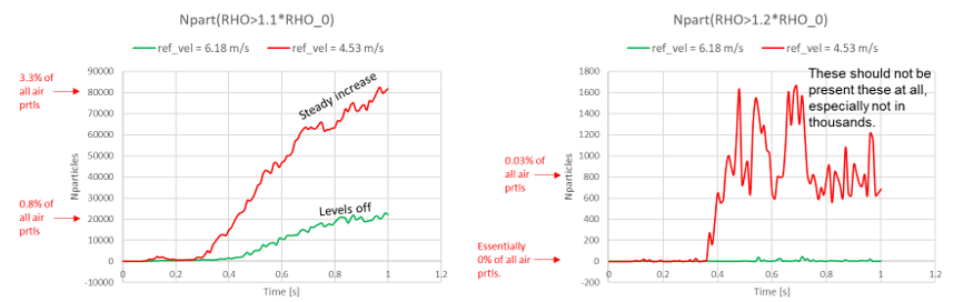
Figure 1. . Information file plots of particles exceeding 10 and 20 percent of . The red lines show results from the case with ref_vel = 4.53 m/s and the green line shows results from the simulation with ref_vel = 6.18 m/s.
While by no means is this type of analysis an absolute or universal measure of simulation quality, it is an extremely useful tool and can be a good starting point to troubleshoot a simulation.
For more information on diagnosing a simulation which has problems, see Troubleshoot a Simulation.