Work Flow

The following describes the intended work flow and some general tips for going through the steps to run a simulation using BasicFEA.

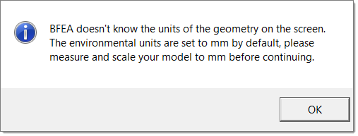
BasicFEA will read the unit system of most geometry files on import and set the working units appropriately. If you get the message shown below it means that BasicFEA was not able to determine the unit system from the geometry file. The default units in the BasicFEA environment are set to mm tonne K N MPa so any new material, load or mesh size are all defined in those units. It is important to match the geometry to the BasicFEA environment before continuing.

basicfea_warning

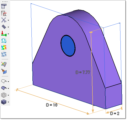
A good first step when starting an analysis is to measure the model. This will give you a feel for the size and is a good check to make sure the units make sense. Click the icon on the toolbar to enter into dimension mode. While in this mode you can simply view the global X,Y,Z bounding box or select your own points to measure.

basicfea_dimension_mode

BasicFEA will read the units from most imported geometry, but if unable to determine the units, or if they are in a set of unsupported units, the Scale model only option in the BasicFEA browser allows you to easily convert only the geometry from units -> units. Right-click anywhere inside the BasicFEA browser and click the Scale model only option.

Switching units in BasicFEA will update the entire model, so use the Scale model only option to match your model to the working units listed at the top of the browser. Separate scale factors can also be applied to the geometry only in order to get a matching set of units between geometry and the rest of the BasicFEA environment.

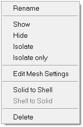
Analyzing parts made of sheet metal can sometimes be challenging due to the nature of the thin, solid geometry. The solution for these types of parts is to find the “midsurface” of the 3D geometry and operate on that with 2D shell elements that carry the representative thickness. Depending on the type of geometry you are importing, BasicFEA has the following options for Solid to Shell midsurfacing:

solid_to_shell_option

3D Solid CAD

•

If the part is considered a thin solid, you have the option to midsurface the part. This option is called Solid to Shell in BasicFEA. Once midsurfaced, you are left with 2D surface CAD and a thickness representing the midsurfaced dimension. If you run this option within BasicFEA, it saves the solid data, so you can run Shell to Solid and get the solid part back.

•	If the part is a cast part and is not thin, then it is not a good candidate for Solid to Shell midsurfacing. In this case the option is removed, and BasicFEA operates on the solid part.

2D Surface CAD

•

If you have already used some of the advanced midsurfacing tools in HyperMesh, or have 2D surface CAD from another source, you can import it. If it has thickness metadata available, BasicFEA will assign the thickness to the part. If not, it will use the average element size algorithm to give you a starting thickness for each part so that the model can run through.

Solid parts in the BasicFEA browser are represented by the icon and have their material displayed as a child. Shell parts are represented by the icon and have the material child along with a thickness editor that changes the thickness for the entire part.

Meshing is something that is done behind the scenes with BasicFEA. Mesh size and type are automatically generated on import and the elements are added right before the analysis is submitted.

If you want to change the mesh settings, that ability is offered on the global scale and for each individual part.

None of the setup for BasicFEA is dependent on a mesh. HyperMesh offers a great deal of meshing options and techniques. At anytime a model generated in BasicFEA can be brought back into HyperMesh and meshed separately by clicking the icon. Moving from BasicFEA to the HyperMesh client ensures that you have a running model to start with before continuing with advanced pre-processing.

BasicFEA supports two types of contact: tied and sliding. To create a contact choose New Tied Contact or New Sliding Contact from the Contacts right-click context menu. The contact definition will be automatically created, leaving you to choose the main and secondary parts. Choose from the list of parts or pick on the screen.

At any time, tied contact can be switched to sliding contact, and vice versa. You can input friction values for sliding contacts. Tied contacts do not have friction.

Auto-contact is a simple way to define contact throughout your model. Selecting Auto-contact from the Contacts folder will search through each part in your model and define a tied contact on parts within an automatic volume based tolerance. It is recommended to review each contact before submitting an analysis. After running an auto-contact, the newly created tied contact pairs can be changed, deleted or switched to sliding to perform a non-linear sliding contact analysis.

BasicFEA supports the following loadstep types:

•

Linear Static: Linear static analysis can be used to determine the effects of static loads on structures using the stiffness method of finite element analysis to solve for the resulting displacements of the structural grids. From the displacements, the element forces, stresses and strains are then calculated. In order to achieve meaningful results some limitations must be noted while setting up a problem. Material stresses must remain in the elastic region. This means that the implied loading must not cause stresses larger than the yield point of each material. In addition, the resulting displacements must be small. This implies the applied loading must not cause large deflections and large rotations leading to geometric non-linearities. Contact between parts must be linear (small sliding). Large sliding contact is only possible through non-linear methods. The problem must remain static and all degrees of freedom must be accounted for while solving a problem. Mechanisms will cause the solver to error with a proper message.

The Linear Static loadstep type in BasicFEA allows you to load your model in the linear space using constraints and distributed loads applied to geometry.

•

Normal Modes: Normal modes analysis, also called eigenvalue analysis or eigenvalue extraction, is a technique used to calculate the vibration shapes and associated frequencies that a structure will exhibit. It is important to know these frequencies because if cyclic loads are applied at these frequencies, the structure can go into a resonance condition that will lead to catastrophic failure. It is also important to know the shapes in order to make sure that loads are not applied at points that will cause the resonance condition.

normal_modes

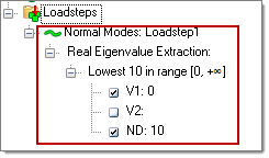
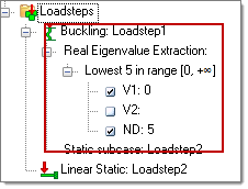
Frequency ranges and the number of desired roots are all controlled within the details of each Normal Modes loadstep. Without a constraint defined in the loadstep a free-free boundary condition is assumed, and by default the first six modes found will be the rigid body modes.

•

Buckling: Linear buckling analysis can be used to determine the maximum or critical loading of a structure prior to its instability or collapse. The problem of linear buckling in finite element analysis is solved by first applying a reference level of loading to the structure and performing a simple linear static analysis to obtain the stresses. From these stresses, the geometric stiffness matrix is calculated. The geometric stiffness matrix along with the mass and stiffness matrix of the structure are then used in an eigenvalue analysis which calculates the buckling load factors, relative to the reference static load. The lowest reported buckling mode factor represents the fraction of the load defined in the referenced Linear Static loadstep that will buckle the structure.

buckling

•	Non-Linear Quasi-Static: The Non-Linear Quasi-Static loadstep in BasicFEA is solving a non-linear quasi-static analysis. The solution supports both small and large deformation theory problems.

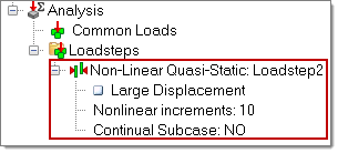
Small deformation theory is used in the solution of nonlinear problems, similar to the way it is used with linear static analysis. Small deformation theory means that strains should be within linear elasticity range, and rotations within small rotation range. This also means that there is no update of gap/contact element locations or orientation due to the deformations. They remain the same throughout the nonlinear computations.

Large deformation theory is used in nonlinear problems by enabling the large displacement option (LGDISP) which allows for non-linear load-response relationships and structural large displacements. Strains can go beyond the linear elastic range and into the plastic region given a valid material definition and rotations can be larger within the range.

Continual subcase allows you to select a previous nonlinear subcase to continue the solution from one subcase to another.

basicfea_sliding_contact

The same loading is available for a Non-Linear Quasi-Static loadstep that is available for linear statics. Before running the analysis make sure to choose which contact definitions are sliding and which are tied. While running a Non-Linear Quasi-Static loadstep containing sliding contacts a search is conducted for open and closed contact based on the loading conditions. Tied contacts simply tie two parts together. If a sliding contact is defined for a linear type loadstep, it will act as a tied contact.

•

Fatigue: Fatigue analysis, using S-N (stress-life) and E-N (strain-life) approaches for predicting the life (number of loading cycles) of a structure under cyclical loading can be setup using BasicFEA. The stress-life method works well in predicting fatigue life when the stress level in the structure falls mostly in the elastic range. Under such cyclical loading conditions, the structure typically can withstand a large number of loading cycles; this is known as high-cycle fatigue. When the cyclical strains extend into plastic strain range, the fatigue endurance of the structure typically decreases significantly; this is characterized as low-cycle fatigue. The generally accepted transition point between high-cycle and low-cycle fatigue is around 10,000 loading cycles. For low-cycle fatigue prediction, the strain-life (E-N) method is applied, with plastic strains being considered as an important factor in the damage calculation.

fatigue

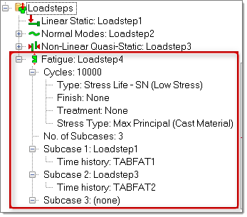
BasicFEA allows for the selection of both linear static and non-linear quasi-static subcases. Additionally, you can select up to 10 total subcases for cycling between. There is also the ability to specify time history data through direct input or import. Additional options are available within the BasicFEA browser, although not every solver option is covered. For full control of the fatigue loadstep, switch to the OptiStruct user profile, and consult the OptiStruct User Guide for more information.

Cycles	This is the number of repeats of the loading sequence. Since the loading is simply a full loading and unloading of one linear static loadstep, or the loading and unloading of two linear static loadsteps consecutively, this will define the length of the event.
Type	Stress Life (SN) is typically used for low stress, high cycle fatigue simulations. Strain Life (EN) is typically used for high stress, low cycle fatigue simulations. Please see the OptiStruct User’s Guide for more information.
Finish	Surface condition is an extremely important factor influencing fatigue strength, as fatigue failures nucleate at the surface. Surface finish and treatment factors are considered to correct the fatigue analysis results.
Treatment	Surface treatment can improve the fatigue strength of components. NITRIDED, SHOT-PEENED and COLD-ROLLED are considered for surface treatment correction. In general cases, the total correction factor is Csur = Ctreat * Cfinish. If treatment type is NITRIDED, then the total correction is Csur = 2.0 * Cfinish (Ctreat = 2.0). If treatment type is SHOT-PEENED or COLD-ROLLED, then the total correction is Csur = 1.0. It means BasicFEA will ignore the effect of surface finish. The fatigue endurance limit FL will be modified by Csur as: FL' = FL * Csur. For two segment S-N curve, the stress at the transition point is also modified by multiplying by Csur.
No. of Subcases	Allows you to select the number of subcases to be evaluated in fatigue simulation. The limit is 10.
Stress Type	BasicFEA offers the choice between Max Principal (for brittle materials) and Signed VonMises (for ductile materials). More stress types are available in the OptiStruct user profile. For Stress Life, a combined stress value is used. For Strain Life, a combined strain value is used. For Strain Life, shear strain components are engineering shear strain (two times tensor shear strain).
Static Subcase 1	At least one linear static or non-linear quasi-static loadstep must be selected before the fatigue simulation can be solved. One loading sequence is the full loading and unloading of this linear static loadstep, and then is repeated by the number of cycles.
Static Subcase 2	If two or more loadsteps are selected, the loading sequence is the full loading and unloading of Static Subcase 1 followed by the full loading and unloading of Static Subcase 2. This is then repeated by the number of cycles.

A Common Loads folder is available in the BasicFEA browser by default. Loads in this folder will be applied to all loadsteps.

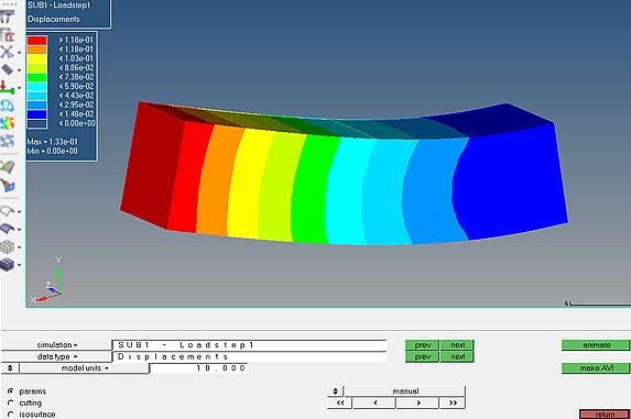
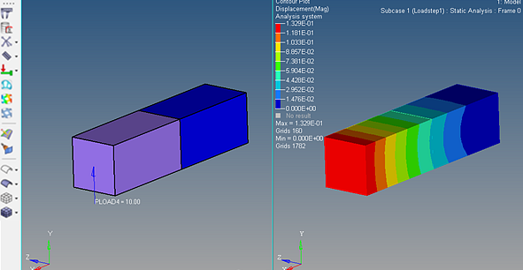
Post-processing in BasicFEA is limited to what exists in HyperMesh post. Producing simple stress and displacement contour and vector plots is available in the Contour and Vector Plot panels. For simple animations and deformed shapes, the Deformed panel allows you some flexibility.

basicfea_postprocessing

If the post-processing is not sufficient in BasicFEA, clicking the icon takes you to the HyperView client, which may be more appropriate for advanced post-processing and report generation.

basicfea_postprocessing2

Work Flow

Work Flow

Work Flow

3D Solid CAD

2D Surface CAD

See Also: