Example for Using the Phase Centre Utility
The different methods provided by the phase centre application macro to calculate the phase centre of a simple horn antenna are utilised and the results are compared to illustrate their differences.
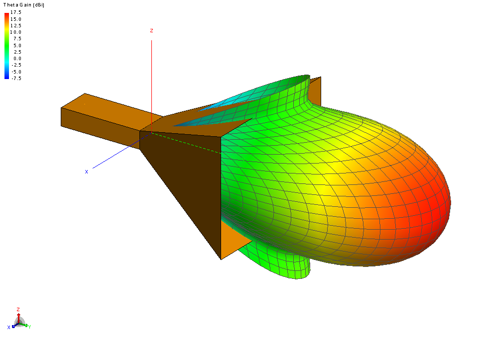
Figure 1. Horn model and θ component of the far field.
It is clear from the image that the horn is not an isotropic radiator, but over a small section of the main beam it can be considered to be an approximate isotropic radiator. This is the assumption that is made during the phase centre calculation. The phase centre calculation determines the origin of such a “fictitious” isotropic radiator.
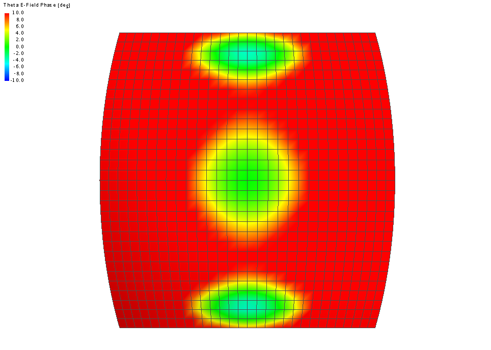
Figure 2. A 3D view plot of the phase of the far field of the horn antenna example.
Phase Calculation Method 1 (Phase Centre at a Single Point)
The first phase calculation method will now be used to calculate phase centre relative to the centre of the main beam for the θ component. The far field result application macro is listed below:
local phase_centre = require("phase_centre_utility")
farfield = pf.farfield.get("Feeding_a_Horn_Antenna_Pin_Feed.StandardConfiguration1.FarField1")

function ff_component(ff)
-- extracts the correct ff component
    return ff.theta
end

-- Calculate the phase centre
pc = phase_centre.phase_centre_m1(farfield, ff_component)
print("The phase centre is located at")
print("X =" .. pc[1])
print("Y =" .. pc[2])
print("Z =" .. pc[3])

-- Move the far field origin to the calculated phase centre
phase_centre.move_far_field_origin(farfield, {pc[1], pc[2], pc[3]})

-- Set phase to zero at centre of the beam
-- This makes visualisation and comparison easier and is not required when only interested in the phase centre
farfield = phase_centre.normalise_ff_phase(farfield, ff_component)
return farfield
The image (below) shows the resulting phase distribution when the far field is located at the phase centre calculated by the first method. We can see a large green area where the phase is close to zero, but then the phase deviates quickly (blue region).
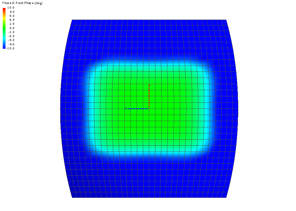
Figure 3. A 3D view plot of the phase variation of the far field of the horn antenna example at the phase centre calculated using the first method.
Phase Calculation Method 2 (Minimize Maximum Phase Deviation)
Here the second phase centre calculation method is used to calculate the phase centre of the θ component. Since this method tries to find the point that minimises the phase variation over the entire far field request, this method is more suited to smaller far field requests. This example illustrates what can be calculated, but it would have performed better if the far field area was reduced. The application macro used to calculate the far field phase is shown below:
local phase_centre = require("phase_centre_utility")

farfield = pf.farfield.get("Feeding_a_Horn_Antenna_Pin_Feed.StandardConfiguration1.FarField1")

function ff_component(ff)
-- extracts the correct ff component
    return ff.theta
end

-- Use the first phase centre calculation method as the initial phase centre (starting point)
pc = phase_centre.phase_centre_m1(farfield, ff_component)
phase_centre.move_far_field_origin(farfield, {pc[1], pc[2], pc[3]})

-- Loop a few times calculating the phase centre in a volume. With each
-- iteration we reduce the size of the volume and also the spacing between
-- sample points. This is done to improve the speed of the calculation.
num_it = 5
refinement = 5
for it = 1, num_it do
    pc = phase_centre.phase_centre_m2(farfield, ff_component,1/(refinement^(it-1)),6)
    phase_centre.move_far_field_origin(farfield, {pc[1], pc[2], pc[3]})
end

print("The phase centre is located at")
print("X =" .. pc[1])
print("Y =" .. pc[2])
print("Z =" .. pc[3])

-- Set phase to zero at centre of the beam
-- This makes visualisation and comparison easier and is not required when only interested in the phase centre
farfield = phase_centre.normalise_ff_phase(farfield, ff_component)

return farfield
The following image illustrates the phase variation for the far field located at the phase centre calculated by the second method. We can see the phase varies considerably, but that the area with a phase close to zero is larger and the phase does not change as dramatically as in the other images.
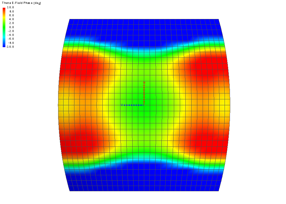
Figure 4. A 3D view plot of the phase variation of the far field of the horn antenna example at the phase centre calculated using the second method.