Temperature coefficient
Introduction
The models provided for B(H) curves, depending on the temperature, with exponential decay, are defined using:
- the previous models provided for soft materials
- a COEF(T) temperature coefficient, built on the basis of two exponential functions (detailed description is in following blocks)
Temperature coefficient
The COEF(T) temperature coefficient is defined by two exponentials:
- the first, with a negative curvature, is used when this coefficient ranges from 1 to 0.1 (T < T1)
- the second, with a positive curvature, is utilized in the neighborhood of the Curie point, when this coefficient ranges from 0.1 to 0 (T < T1 )
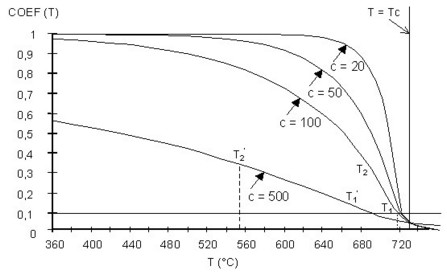
The shape of the COEF(T) temperature coefficient is represented in the figure below.
Mathematical model
The COEF(T) temperature coefficient is defined in the following way:
for T < T1: ![]()
where for the temperature T1 we have COEF1(T1) = 0.1
The last relationship can be equally written as: T1 -Tc =C ln 0.9
for T > T1: ![]()
where the quantity T2 has the value so that the connection of the two exponentials could be effected in T1, i.e. COEF2(T1) = 0.1
This last condition can be equally written as: T2 -T1 =0.1C ln 0.1
where:
- Tc is the Curie temperature °C
- C is the temperature constant °C
Exact mathematic expression
The expression of COEF(T) used above between 1 and 0,1 is approximate. The accurate expression :

As Tc is elevated, around 1000 K, we use the approximation:
![]()
And at Td0 = 0°C:
![]()
Example
The shape of the COEF(T) function is represented in the figure below.
The decrease of the COEF(T) coefficient is more or less rapid following the value of the C temperature constant supplied by the user.
