MV-9001: Simple Pendulum Tutorial

In this tutorial, you will learn how to model a simple 1 DOF mechanism using the Msolve MotionSolve Python API.

If you are running this tutorial as IPython notebook, you can interactively execute each code cell by clicking SHIFT-ENTER. The output of the Python code (if any) will be displayed and the execution will jump to the next cell.

The image below is a graphical representation of the system that you are going to build.

Figure 1.

A rigid body is suspended by a mass-less wire and is connected to the ground via a hinge joint. The only force acting on the system is gravity, directed along the negative vertical direction. The simulation shows a part swinging from its initial resting position. There is no friction force in the joint, nor any type of energy dissipating force acting on the part, therefore the ball reaches 180 degrees of angular displacement for each full swing.

You will examine the reaction force in the joint.

Load the Msolve Module

Load the msolve module, which is done by issuing this command:

In [1]: from msolve import*

The above command requires the msolve module to be in your computer path. Assuming the above is successful, you have imported the msolve names into the current namespace. This means that you have access to all classes and functions defined in msolve and you can start creating the simple pendulum.

Create a Model

To create the pendulum mechanism, you must first create a model. A model is nothing but a container that serves as a parent for all the entities. The model class takes a keyword argument to specify the output file name for MotionSolve. You can use the name 'pendulum'.

Issue this command:

In [2]: model = Model(output='pendulum')

MotionSolve creates a series of output files (such as .mrf, .abf and .h3d) using pendulum as the root name.

Add Units and Gravity

After creating a model, you can add details, units, and other entities such as gravity and ground. Most entities have default properties. For example, when you create the solver unit set without specifying arguments, you are essentially creating SI units.

Issue this command:
```
In [3]: units= Units () 
```
Since you want to model in mmks, modify the length property of the units and assign a value of "MILLIMETERS". You can perform a simple direct assignment:.
```
In [4]: units.length="MILLIMETER"
```
Similarly, you can create the gravitational acceleration field with the Accgrav class.
```
In [5]: gravity=Accgrav(kgrav=-9810)
```
Notice the result of the Accgrav creation is stored in a variable called gravity. That is the name that appears to the left of the equal sign. This is now a Python variable in the current namespace and, as such, can be used anywhere in the scope.

Note that in msolve class names, use the CapWords convention and be aware that you can use the Python help system to learn about each msolve class, its use, and properties. Complete the steps below as an example.

To interact with the Accgrav class, call the help ( ) function with the class name as the input argument.
```
In [6]: help(Accgrav)
Help on class Accgrav in module msolve.Model:
class Accgrav(Force)
 |  Accgrav defines the acceleration due to gravity along the global X, Y, and Z directions.
 |
 |  Method resolution order:
 |      Accgrav
 |      Force
 |      msolve.Base.SolverObject
 |      __builtin__.object
 |
 |  Methods defined here:
 |
 |  sendToSolver(self)
 |      Send the object to the solver
 |
 |  setSolverValue(self, name, value)
 |      Set the property 'name' to 'value' between simulations
 |
 |  ----------------------------------------------------------------------
 |  Data descriptors defined here:
 |
 |  igrav
 |      Gravity in the global X direction
 |      Type=Double, Optional, Default=0
 |      Modifiable during simulation
 |
 |  jgrav
 |      Gravity in the global Y direction
 |      Type=Double, Optional, Default=0
 |      Modifiable during simulation
 |
 |  kgrav
 |      Gravity in the global Z direction
 |      Type=Double, Optional, Default=0
 |      Modifiable during simulation
```
A lot of information is displayed when the help function is called. The most important piece of information is the description of the class and its properties. For example, data descriptors are defined in the code below:
```
igrav
    Gravity in the global X direction
    Type=Double, Optional, Default=0
    Modifiable during simulation
```
In msolve, creating a class instance always returns an object. This gives you the ability to reference the object using its name, gravity in this case. You can use gravity and its properties anywhere in the model. For example, you can modify its properties during the model building phase, or between MotionSolve simulations. The benefits of this approach are illustrated later in this tutorial.

As a general rule, it's useful to store the objects being created using local variables, especially if they will be modified or referenced elsewhere. At this point, you can proceed with the model creation.
Create the ground part, use the Part class, and specify the ground Boolean attribute as 'False'.
```
In [7]: ground=Part(ground=True) 
```

Define Points

Some models in MBS are defined using points. Points are a special auxiliary object with an x, y, z location and a handful of convenient methods. They are a powerful way to define a mechanism and can be used anywhere in the model where an X,Y,Z quantity is needed (for example, to position a part or position a marker origin).

In this example, use points to locate various objects (such as markers) in the three dimensional space. You can use points when defining marker locations and orientations.

To create a point at the global origin, do not include an argument, as not having an argument in the Point class signifies that the x,y,z coordinates are set to the default values of 0,0,0. Issue the following command:

In [8]: p0=Point()

Create Markers

You can use this point to locate the origin of the ground marker. A marker is defined by a geometric point in space and a set of three mutually perpendicular coordinate axes emanating from that point.

In the marker class, the property qp corresponds to the location of the marker origin in the body reference frame. Since you are using ground as the body, the qp propery is the location of the marker in the global reference frame. Use the zp, xp method to orient the Z and X axes.

In the command below, supply a point in space used to orient each of the two axes, the third being automatically computed as an orthogonal right handed coordinate system.
```
In [9]: ground_mar=Marker (body=ground, qp=p0, zp=[0,100,0], xp=[100,0,0]) 
```
Now you can create the pendulum body. It's a rigid part with a mass of 2kg and some nominal inertia properties.
```
In [10]: part=Part(mass=2.0, ip=[1e3,1e3,1e3]) 
```
Optional: If you type part. and the TAB key in a code cell, you will be able to see all the functions and properties applicable to part as a drop down list.

Verify the Part Creation

Every entity can be interactively validated. This is a way to help ensure that only correct models are simulated. The part that you created in the code cell above has mass properties but it does not have a Center of Mass marker. Therefore, it is incorrect. You can

Verify the part by calling the validate function:

In [11]: part.validate() 
Part/2
ERROR:: Mass is specified but cm is not specified.
ERROR:: There are no markers on this part.
Out[11]:
False

The error message tells you the part CM is missing.

Rectify this issue by creating the part CM marker at position (100, 0, 0). This point represents the location of the pendulum part.

In [12]: p1 = Point(100,0,0)
# create the marker as the part.cm 
# note that the '.' operator allows us to define a the 'cm' property of the part object. 
# the marker will be positioned at (100,0,0), the X axis is pointing towards the point (200, 0,0) 
# and the z axis points to (200, 100, 0)
 
part.cm = Marker(body=part, qp=p1, zp=[200,100,0], xp=[200,0,0])

Create a Geometry Object

For animation purposes, you can create a geometry object, a sphere in this case. According to the documentation, a sphere requires a center marker and a radius.

Issue this command:

In [13]: sphere=Sphere (cm=part.cm, radius=20)

Add Joints and Requests

You will need to properly constraint our sphere, otherwise it will fall. A pendulum can be modeled using a revolute joint at the hinge point p0. This will effectively capture the undeformable, infinitely rigid mass-less connection of the pendulum body to ground. The revolute joint will connect two markers, one on the pendulum sphere and one on ground, and these markers need to be properly positioned in the three dimensional space.

A requirement of the revolute joints is that the i and j markers need to be coincident and need to have their Z axes properly aligned.

You will also create a request. Requests define output channels in MotionSolve and are written to MotionSolve output files so that they may be used for plotting and signal processing by HyperGraph. Requests can be defined using runtime expressions, built-in functions (MOTION, FORCE, FIELD, and so on,) or user written functions.

In this case, you can create a force request using the predefined "FORCE" method and create another request tracking angular displacement using the AX MotionSolve runtime function. AX measures the angular displacement in radians between two markers.

Issue the following command:

In [14]: joint = Joint(type="REVOLUTE", i=ground_mar, j=Marker(body=part, qp=p0, xp=[100,0,0], zp=[0,100,0]))
force_req = Request(type="FORCE", i=joint.i, j=joint.j, rm=joint.i)
angle_req = Request(f1="RTOD*AX({I}, {J})".format(I=joint.i.id, J=joint.j.id),                    
                    f2="RTOD*AY({I}, {J})".format(I=joint.i.id, J=joint.j.id),
                    f3="RTOD*AZ({I}, {J})".format(I=joint.i.id, J=joint.j.id))

Call Sforce to calculate the contact force as the ball moves. The input function should be a MotionSolve expression and the z axis of marker j defines the direction that the force applies.

In [15]: input_function =
"IMPACT(DZ({I}, {J}, {J}),VZ({I}, {J}, {J}),{G},{K},{E},{C},{D})"
.
format( I=marker_i.id,J=marker_j.id, K=5e9, G=0.00, E=1.0, C=0.8e5, D=0.0 )
contact_force = Sforce(i = marker_i.id, j = marker_j.id,
type=
"TRANSLATION"
, function = input_function)

Run the Simulation

At this point, you are ready to run a transient analysis. The simulate method in invoked on the MBS model. A validation process is performed on each of the entities that make up the model. This is a necessary step to ensure that only correct models are being simulated. Note that the simulate command can be invoked with an optional flag returnResults set to True. This stores the results of the simulation into a run container for further post-processing, as shown in the following code.

Issue the following command:

In [16]: run=model.simulate (type="TRANSIENT", returnResults=True, end=2, dtout=.01)

You can easily modify the part mass property by changing its value with a direct assignment:
```
In [17]: part.mass= 12
```
At this point you can run another simulation, starting from the end of the previous analysis. To do that, simply issue a new simulate command and specify an end time of four seconds. Note that this simulation is done with the new part mass, so you should be able to see the effect of that in the joint reaction forces.
```
In [18]: run=model.simulate (type="TRANSIENT", returnResults=True, end=4, dtout=.01)
```
In the following command, you are extracting the force_req from the run container. The purpose is to have a convenient data structure for extracting time varying results.
```
In [19]: force=run.getObject (force_req)
```
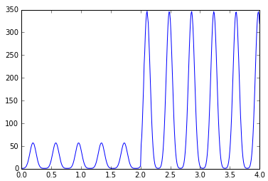
You can use the force object to plot the longitudinal reaction force Fx. To do so, you are using the matplotlib module available in the IPython notebook. The plot is displayed inline. You can see how the mass modification at time = 2 sec affects the magnitude of the reaction force, generating a peak of 350N.
```
In [20]: %matplotlib inline
from matplotlibimport
pyplot pyplot.plot (force.times, force.getComponent (2), label=force.labels[2])
```
Figure 2. Out[20]: [<matplotlib.lines.Line2D at 0x7142860>]
Similarly, you can plot the rotation angle. A generic runtime expression was used in the angular displacement request, so you need to get the right component that corresponds to the AY (angle about the Y axis of the marker j of the angle request.
```
In [21]: angle = run.getObject(angle_req)
pyplot.plot (angle.times, angle.getComponent(2), label="angle [deg]")
```
Figure 3. Out[21]: [<matplotlib.lines.Line2D at 0x72c8fd0>]
The angular displacement is a simple harmonic function and the pendulum reaches 180 degrees because there are no dissipative forces such as viscous friction in the joint. Note that the frequency of oscillation is governed by these equations:(1) $T = 2 π \sqrt{\frac{L}{g}}$ (2) $f = \frac{1}{T}$
As visible from the plot above, the mass swings with a frequency of about 1.5Hz. The generateOutput() function called below creates a MotionSolve *.plt file and H3D animation files for visualization in HyperView and HyperView Player.
```
In [22]: model.generateOutput()
```

In conclusion, you have learned how to create a simple pendulum model, run transient simulations, and plot results.