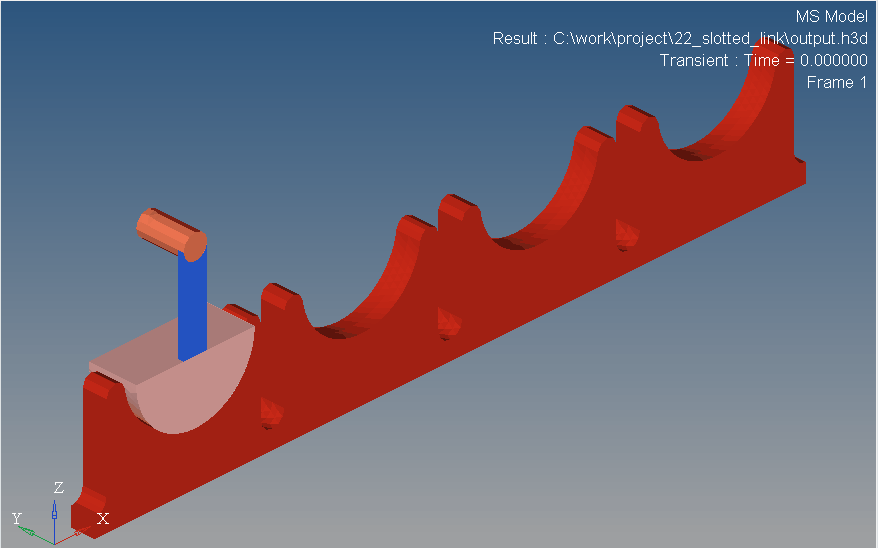
MV-9002: Slotted Link Tutorial
In this tutorial, you will learn how to import geometry and build a Poisson Contact using the msolve MotionSolve Python API.
If you are running this tutorial as IPython notebook, you can interactively execute each code cell by clicking SHIFT-ENTER. The output of the Python code (if any) is displayed and the execution jumps to the next cell. If you want to run it, you also need to make sure that the file slotted_link.fem is in the folder.
Load the Msolve Module
In [1]: from msolve import*The above command requires the msolve module to be in your computer path. Assuming the above is successful, you have now imported the msolve names into the current namespace. This means that you have access to all the classes and functions defined in msolve and you can start creating the bouncing ball case.
Create a Model
To create the pendulum mechanism, you must first create a model. A model is nothing but a container that serves as a parent for all of the entities.
In [2]: model = Model() Add Units and Gravity
Add Parts
Next, you can create four parts representing the link, cam, pin, and slotted link. You can also specify the mass, initial property, and the center of mass for the part. This information would not be imported to MotionSolve from CAD or FEM file automatically.
In [6]: link = Part(cm=Marker(),mass = 0.0526,ip=[20.0844,21.7819,1.9169,0,0,0])
link.cm.qp = [0, -17.499994784, 33.609856169]
pin = Part(cm=Marker(),mass = 0.0972, ip = [15.3742, 4.8085, 15.37, 0,0,0])
pin.cm.qp = [0,-0.000001527,74.999999124]
cam = Part(cm=Marker(),mass = 1.2159, ip = [372.14,961.3416,913.45,0,0,0])
cam.cm.qp = [0,0,-21.22]
slotted_link = Part(cm=Marker(),mass = 5.8943,ip = [3721.7065,1.8e5,1.7689e5,0,0,0])
slotted_link.cm.qp = [224.988, 0, -63.813495]
Define Markers for Geometry
Before importing the geometry, you need to define the marker on the part that the geometry is linked to. You cannot use cm marker in this case; the position of nodes in the FEM is measured in the global reference frame while the cm marker represents a local reference for the part. So, you need to create four markers that coincide with global origin.
In [7]: link_geo_marker = Marker(part = link)
pin_geo_marker = Marker(part = pin)
cam_geo_marker = Marker(part = cam)
slotted_link_geo_marker = Marker(part = slotted_link)
Import Geometry
Now you can import geometry for the part. To do so, create four external instances. The class External is created to help users import a CAD file or an FEM file. If the file imported has multiple components, you can extract them one-by-one by specifying the 'element' property. When the CAD file is imported, you can improve the mesh by increasing the value of 'refinement_level'. The example below shows how external instances are created in this case:
In [8]: link_geo = External(rm = link_geo_marker, file ="slotted_link.fem",
                    element=["Link"], refinement_level = 0)
pin_geo  = External(rm = pin_geo_marker,  file ="slotted_link.fem",
                    element=["Pin"], refinement_level = 0)
cam_geo  = External(rm = cam_geo_marker, file ="slotted_link.fem",
                    element=["Cam"], refinement_level = 0)
slotted_link_geo = External(rm = slotted_link_geo_marker, file ="slotted_link.fem",
                    element=["Slotted_Link"], refinement_level = 0)
Add Joints
The next step is to create the joints between different parts. Two fixed joints are created: one between the pin and the link, and the other connecting the link and the cam. For a fixed joint, the i marker and j marker should be coincident with their x,y,z axis aligned.
Add Motion
The motion can be created by creating an instance of Motion in msolve. You can change the pattern of motion by specifying the property 'function'. The property 'function' should be a MotionSolve expression.
In [12]: cam_pivot_motion = Motion(joint=cam_pivot_revolute, jtype="ROTATION",dtype=
"DISPLACEMENT",function='360d*TIME')
Add Contact
The last step is to create contact between the geometries that you imported. Two Poisson contacts are created here: one between the cam and slotted link, and the other between pin and slotted link.
In [13]: cam_slotted_contact = Contact(igeom=cam_geo,jgeom=slotted_link_geo,type="POISSON",
                             restitution_coefficient=0.5,penalty=1e5)
pin_slotted_contact = Contact(igeom=pin_geo,jgeom=slotted_link_geo,type="POISSON",
                              restitution_coefficient=0.5,penalty=1e5)
Create Requests
Before running the model, create requests that track the contact force and the penetration depth. The result can be plotted using pyplot.
In [14]:#forceRequest = Request(f2="FX({I})".format(I=slotted_link_geo_marker.id))
forceRequest = Request(f1="CONTACT({ID},{JFLAG},{COMP},{RM})".format(ID=cam_slotted_contact.id,
                        JFLAG=1,COMP=1,RM=0),
                       f2="CONTACT({ID},{JFLAG},{COMP},{RM})".format(ID=pin_slotted_contact.id,
                        JFLAG=1,COMP=1,RM=0))
depthRequest = Request(f1="CONTACT({ID},{INDEX},{RM})".format(ID=cam_slotted_contact.id,
                        INDEX=1,RM=0),
                       f2="CONTACT({ID},{INDEX},{RM})".format(ID=pin_slotted_contact.id,
                        INDEX=1,RM=0))
Run the Simulation
At this point you are ready to run a transient analysis. The simulate method is invoked on the MBS model. A validation process is performed on each of the entities that make up the model. This is a necessary step to ensure that only correct models are being simulated. Note that the simulate command can be invoked with an optional flag, returnResults, set to True. This stores the results of the simulation into a run container for further post-processing, as shown below.
You can also generate an output file that can be imported into MotionView for animation.
In [15]: run=model.simulate(type="DYNAMIC", returnResults=True,
end=3, steps = 3000)
model.generateOutput()
Generate a Plot and Animation
%matplotlib inline
force = run.getObject(forceRequest)
depth = run.getObject(depthRequest)
from matplotlib import pyplot
pyplot.subplot(2,1,1)
pyplot.plot(force.times, force.get
Component(0),'r',force.times, force.getComponent(1))
pyplot.title("Contact Force Magnitude")
pyplot.xlabel("Time(s)")
pyplot.ylabel("Contact Force (N)")
pyplot.grid(True)
pyplot.legend(["Cam-Slotted Contact","Pin-Slotted Contact"],loc="upper left",prop={'size':8})
pyplot.subplot(2,1,2)
pyplot.plot(depth.times, depth.getComponent(0),'r',depth.times, depth.getComponent(1))
pyplot.title("Maximum Penetration Depth")
pyplot.xlabel("Time(s)")
pyplot.ylabel("Penetration Depth (m)")
pyplot.grid(True)
pyplot.legend(["Cam-Slotted Contact","Pin-Slotted Contact"],loc="upper left",prop={'size':8})
pyplot.subplots_adjust(hspace=0.5)
pyplot.show()
Figure 1.

Figure 2.