ode15i

Syntax

[t,y] = ode15i(@func,tin,y0,yp0)

[t,y] = ode15i(@func,tin,y0,yp0,options)

[t,y,te,ye,ie] = ode15i(...)

Inputs

func

The system of equations to solve.

tin

The vector of times (or other domain variable) at which to report the solution. If the vector has two elements, then the solver operates in single-step mode and determines the appropriate intermediate steps.

y0

The vector of initial conditions.

yp0

The vector of initial derivative conditions.

options

A struct containing options settings specified via odeset.

The default relative and absolute tolerances are 1.0e-3 and 1.0e-6.

For the option to supply the analytical Jacobian, the function signature should be as follows:

function [dy, dyp] = jacobian(t,y,yp)

where dy and dyp contain the partial derivatives of the system function vector with respect to y and yp, respectively.

Outputs

t

The times at which the solution is computed.

y

The solution matrix, with the solution at each time stored by row.

te

The times at which the 'Events' function recorded a zero value.

ye

The system function values corresponding to each te value.

ie

The index of the event that recorded each zero value.

Example

Solve for the location in a mass spring damper system.

function f = MSD(t,y,yp,v,m,k,c) 
  % y = [x, mD, mS] 
  f = [0, 0, 0]; 
  f(1) = (y(2)-y(3)) - m*yp(1);  % momentum equilibrium        
  f(2) = y(1) - yp(3)/k;         % displacement equilibrium        
  f(3) = (m*v-y(2)) - y(1)*c;    % momentum equilibrium 
end 

m = 1.6; % mass 
v = 1.5; % initial velocity 
k = 1.25; % spring constant      
c = 1.1;  % damping constant 

handle = @(t,y,yp) MSD(t,y,yp,v,m,k,c);      
t = [0:0.2:12]; % time vector      
yi = [0, m*v,0];      
ypi = [v, -c*v, 0.0];      
[t,y] = ode15i(handle,t,yi,ypi);      
x = y(:,1)';
plot(t,x);
xlabel('time');
ylabel('location');

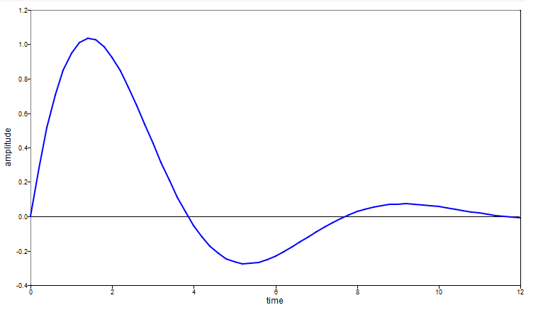
Figure 1. chirp figure 1

Comments

ode15i solves the system using the backward differentiation formula algorithm from the Sundials IDA library.

To pass additional parameters to a function argument, use an anonymous function.

The 'Events' function used with the last three output arguments is specified using odeset.