Exposable Parameters
Learn about the definition, usage, and limitations of exposable parameters.
Selection
Using the exposable function explicitly is one way to define a parameter as exposable. This way, anywhere in the selected Super Block, a parameter can be defined as exposable.
Super Block
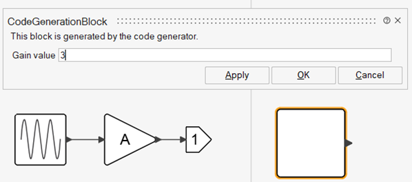
In the following Super Block, the Gain parameter of the Gain block is defined as an exposable parameter named A with the default value 3.
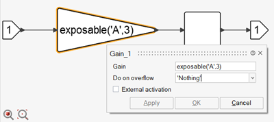
The parameter can also be defined in the Context of the diagram, as follows:
A=exposable(‘A’,3)
and used to define the Gain parameter value of the block. In this case, when code is generated for the Super Block, the parameter A (the gain value) is exposed. The second argument of the exposable function defines the default value of the parameter.
The exposing of the parameter A and its default value can be seen for example by generating the FMU of the Super Block:
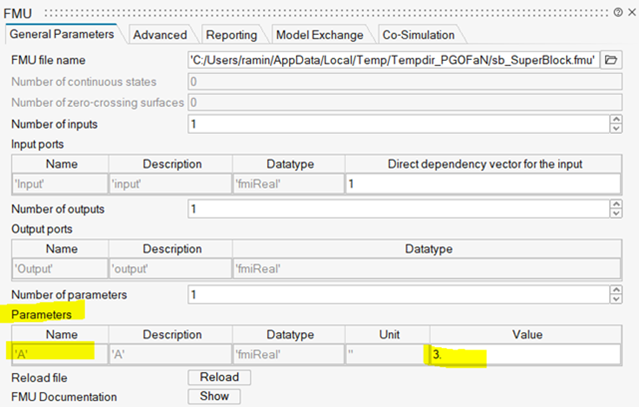
The exposable parameters are defined primarily for code generation purposes, but defining them explicitly using the exposable function affects the simulation of the model as well. Particularly, if a variable with the same name exists in the OML base environment, the exposed parameter takes the value of this variable in the OML base environment at the Model Evaluation phase. So, in the above example, if a variable A is defined having a value of 4 in the OML base environment, then the simulation uses this value for parameter A.
If A is not defined in the OML base, then the simulation runs normally as if A were not exposed (with value 3). The exposable function behaves like the GetFromBase function during the Model Evaluation phase.
This way of designating a parameter as exposable is useful in some cases, for example when a deep level parameter is to be made exposable without having to modify the model, but in most cases it is not the most convenient way of defining exposable parameters. The natural way to select exposable parameters in a non-masked Super Block is to consider as exposable, variables used but not defined inside the Super Block, in the way auto-masking selects the mask parameters. In this approach, a transparent auto-masking operation is used to identify exposable parameters. If a Super Block is already masked, then the exposable parameters are extracted from the expressions defining the mask parameter values.
Therefore, two situations must be considered: generating code for a masked Super Block and generating code for a non-masked Super Block.
Unmasked Super Block
Suppose you select a non-masked Super Block for code generation and a variable A is used inside the Super Block but defined outside of the Super Block. Then A is considered as exposable and its value that is defined outside is considered as its default value. The identification of exposable parameters is done through an implicit transparent auto-masking operation, so if you want to examine the set of exposable parameters, you can temporarily mask the Super Block by performing a manual auto-masking operation.
Unmasked Super Block
The following non-masked Super Block contains a Gain block with the variable A as the parameter value, which is defined in the Initialization script of the model.
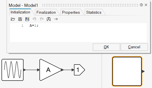
Code generation for this Super Block considers A as exposable with the default value 1. So implicitly, exposable(‘A’,1) is used as the parameter of the Gain block.
Masked Super Block
Suppose the selected Super Block is already masked. Then, the same logic is used to determine the exposable parameters: the Super Block is (re-)masked by auto-masking to determine the exposable parameters.
Masked Super Block
Consider the same Super Block, but masked:
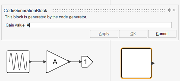
In this case A again is considered exposable, and its default value is taken to be 1. Note that A is considered exposable because the value of the mask parameter is defined as A and not because of the name of the mask parameter (which also happens to be A), which is a local variable inside the Super Block. This means that if the value of the mask parameter is defined numerically:
Similarly, in the following example:

the exposable parameters are B and C (A is not exposable in this case as it is a local variable of the Super Block).
Note that the two methods for defining exposable parameters (via Super Block mask parameters and the explicit use of the exposable function) can be used in the same model. However, the value of masked parameters of the Super Block should not be made exposable using the exposable function. This action would cause redundancy, and the parameter would be rejected by the compiler.
Limitations with Exposable Parameters
Exposable parameters of a Super Block can be used directly to define parameters of the blocks inside the diagram of the Super Block or used inside the Super Block Context to define new parameters. There are several limitations in the usage of exposable parameters.
Exposable parameters can be used in OML expressions involving basic operators (addition, subtraction, multiplication…), matrix extraction and concatenation, and basic math and trigonometric functions. These functions are overloaded to accept exposable parameters. Since the implementation uses operator overloading, expressions including calls to functions including basic operators and overloaded functions are also supported. However, exposable parameters cannot be used in non-overloaded built-in functions. For example, in the implementation of the Chebyshev filter block presented earlier, the parameters of the mask (filter parameters) cannot be exposed because the OML built-in function cheby1 is not overloaded.
Even if an expression involving exposable parameters is valid, it cannot necessarily be used to define any block parameter value. Not all block parameters in Activate libraries accept expressions with exposable parameters. Structural block parameters are clearly excluded, and so are any parameters that affect the size or type of signals. Other block parameters, for the most part, accept expressions with exposable parameters.
Classical Inverted Penulum on a Cart
Consider the problem of the classical inverted pendulum on a cart.
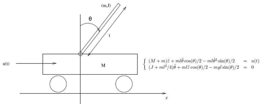
The system state contains the position and speed of the cart, and the angle and angular velocity of the pendulum. State feedback control is used to stabilize the pendulum in the vertical upright position. The model contains a delay block for studying the effect of control delay in the performance of the controller:
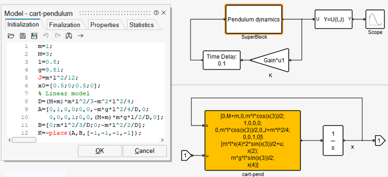
The model of the Pendulum dynamics is placed inside a Super Block. Here various code generation methods are applied to this Super Block, illustrating how the methods work and differ.
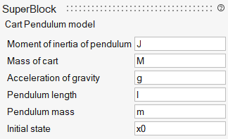
The Super Block has one input (force applied to the cart) and one output (vector containing all four elements of the state). The parameters used inside, and defined outside, are the cart and pendulum masses, M, m, the pendulum length, l, its moment of inertia, J, the initial state x0 (the initial state of the Integrator block) and the gravity constant g. These parameters can be seen by auto-masking the Super Block: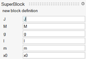
The Super Block can now be used like a regular block, with the mask as the parameter GUI. This GUI can be customized by editing the mask as follows:
Code Generation
The application of code generation to this Super Block, as discussed earlier, exposes all the mask parameters because their values are defined as variables with the same names. The application of the code generators produces a C Custom block with opar parameters x0, J, M, g, l and m, as shown here in the case of the standard code generator:
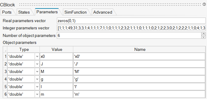
The C Custom block is placed automatically in a masked Super Block with the same parameters. The result here is identical to the case where the code generator is applied to the unmasked Super Block.
Selection of Exposable Parameters to Expose
Parameters that you would want to expose are not necessarily exactly the parameters obtained by masking the Super Block. For example, in the cart-pendulum system, the more natural set of parameters to expose are m, M, l and the initial positions. The moment of inertia is a function of the pendulum mass and length (J=ml2/12) and g=9.81. The full initial state is also often not required; only the initial system positions (cart position and pendulum angles), z0 = x0(1) and θ0 = x0 (3), are considered. To use these as exposed parameters, the mask parameter values of the original system can be modified as follows (the initial velocities are set to zero):
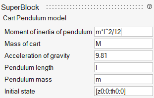
After defining initial values for z0 (z0) and θ0(th0), for example in the Model Initialization script, the application of code generation, as expected, results in the following set of exposed parameters (the values of the exposed parameters here are manually replaced by numerical values):
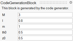
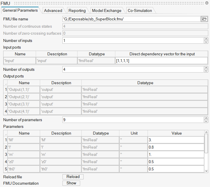
Similarly, the FMU export produces an FMU with the same parameters exposed:
List of Parameters that You Can Expose
In addition to all non-structural Modelica block parameters, the following Activate block parameters are exposable:
| Activate Block | Exposable Parameters |
|---|---|
| Accumulator | x0 |
| Bias | B |
| CompareToConstant | C |
| ConditionalSelect | Thra |
| Constant | C |
| ContStateSpace | x0 |
| ContTransFunc | Num, den |
| Counter | Minim, step |
| Deadzone | lower, upper |
| DFlipFlop | init |
| DLatch | init |
| DiscreteDelay | init_cond, maxim, Initv |
| DiscreteIntegral | x0 |
| DiscrTransFunc | num, den |
| EventDelay | delay |
| EventGenerate | etimes.time{1} |
| FixedDelay | T |
| Gain | gain |
| Horner | coeffs |
| Integral | x0 |
| JKFlipFlop | init |
| LookupTable | xx, yy |
| LookupTable2D | xx, yy, zz |
| LookupTableND | Ff, dimi{i} |
| MatrixGain | gain |
| MathExpression | All parameters used in the expression |
| MatrixExpression | All parameters used in the expression |
| ModuloCounter | ini_state, base, step |
| Power | power |
| PID | Kp, Ki, Kd |
| Ramp | slope, startt, initout |
| RampSaturate | Height, duration, offset, startTime |
| Random | A, B |
| Saturation | upper, lower |
| Sawtooth | Period, up, down |
| SignalGenerator | xx, yy (only scalar double signals, without output derivatives) |
| SineWaveGenerator | M, F, P, offs |
| SquareWaveGenerator | FV, SV, period, dutyCycle, offset |
| SRFlipFlop | init |
| StepGenerator | steptime, iniv, finv |
| Trapezoid | Amplitude, rising, width, falling, period, startTime, offset |
OML Operators and Functions that You Can Apply to Exposable Parameters
Exposable parameters can be used in the computation of the values of exposable block parameters. This computation can be limited to an OML expression or based on the execution of one or more scripts included in Super Block Contexts. Even though there is no explicit limit on the complexity of the resulting expression, the usage should be limited to “simple” expressions; complex expressions may not be efficient to evaluate and may even fail.
Exposable parameters, and other variables depending on exposable parameters, can be matrices of arbitrary sizes. Their usage is supported for the following operators and functions:
- Basic operators:
+ - * / \ .* .\ ./ ^ .^ == ~= > < >= <= & | ‘ .’ : - Matrix row and column concatenations, and matrix extraction (with access via ‘:’ and ‘end’ supported)
- Primitive functions: sin, cos, tan, asin, acos, atan, sinh, cosh, tanh, asinh, acosh, atanh, exp, log, sqrt, min, max, transpose, floor, ceil, round, svd
- Primitive functions returning numeric values: size, length, isvector, isscalar, issquare. Since the sizes of exposable parameters are fixed and do not depend on their values, the output of these functions can be determined at compile time.
- Any OML function that uses only the above operators and functions within its definition, or other OML functions of the same type.
Operators Applied to Exposable Parameters
Suppose X and Y are exposable parameters, then the following expressions and instructions are valid
- X + Y
- Z = X .* Y; sin(Z)^2
- X(1,:) * X(:,1)
- Z = [X, Y]; Z’
- if isscalar(X), Z=X; else Z=Y; end
The last statement is valid because at compile time, it is known whether X is scalar or not based on its default value.
The following expressions and instructions are not valid
- eig(X)
- eye(X,Y)
- if X > 0, Z = X; else Z=0; end
The last statement however can be expressed as an equivalent valid expression as follows
- Z = max(0, X);