Feko is a comprehensive electromagnetic solver with multiple solution methods that is used for electromagnetic field analyses
involving 3D objects of arbitrary shapes.
3D views are used to display and interact with the model. You can zoom, rotate and pan around a 3D model using the keyboard,
mouse or a combination of both. You can use a 3D mouse, specify a view or select specific parts of a model. Multiple 3D
views are supported.
Define field or current data using either far field data, near field data, spherical mode data or PCB current data. Use
the field/current definition when defining an equivalent source or a receiving antenna.
Define a medium with specific material properties, import a predefined medium from the media library or add a medium from
your model to the media library.
Defined media can be applied to the model in various ways. Some media settings are applied to regions, others on faces
and wires. The rules for defining media varies between the different solution methods.
Use a periodic boundary condition (PBC) to analyse infinite periodic structures. A typical application of PBC is to
analyse frequency selective surface (FSS) structures.
Create an arbitrary finite antenna array that consists of an array of contributing elements, either with direct feeds for
each element or via indirect coupling, and solve with the efficient domain Green's function method (DGFM).
Use the windscreen tools to define a curved reference surface constrained by a cloud of points, normals and optional U′V′ parameters. The constrained surface is then used as a reference to create a work surface where windscreen layers and curved
parameterised windscreen antenna elements can be created.
Many electromagnetic compatibility and interference problems involve cables that either radiate, irradiate or cause coupling
into other cables, devices or antennas. Use the cable modelling tool and solver to analyse the coupling and radiation.
For a frequency domain result, the electromagnetic fields and currents are calculated at a single frequency or frequency
range. When the finite difference time domain (FDTD) solver is used, the frequency must be specified to convert the native time domain results to the frequency domain.
The excitation of an antenna is normally specified as a complex voltage, but it may be useful to specify the total radiated
or source power instead. The result is then scaled to yield the desired source power level.
A port is a mathematical representation of where energy can enter (source) or leave a model (sink). Use a port
to add sources and discrete loads to a model.
Obtain multiple solutions for a single model using multiple configurations. Multiple configurations remove the requirement
to create multiple models with different solution requests.
Add a near field boundary request to the model. This type of request allows you to define a cuboidal near field request
where the request points are located on the surface of the cuboid, but you have the option to exclude specific surfaces
(faces).
Use advanced settings to specify the currents taken into account for the calculation of fields or potentials, the
export of near field data and ignoring radiated contributions from impressed sources.
Add an error estimation request. Error estimation is an a-posteriori error indicator which gives feedback on the mesh
quality. The mesh quality is determined by testing the solution against an unconstrained physical test.
Add a model decomposition request to the model. This request exports the surface currents on selected faces to a .sol file. Use a .sol file to define a solution coefficient source in another model.
Calculate the properties of frequency selective surfaces (FSS) in a multilayer scattering scenario by using transmission
and reflection coefficients for plane waves. Use in conjunction with periodic boundary conditions (PBC), multilayer
planar Green's functions or infinite planes for a more efficient solution.
An ideal receiving antenna is a tool that calculates the power that would be received by an ideal antenna. Use this
type of antenna for a more computationally efficient solution.
Add a request to calculate the average absorption over a volume (volume-average SAR) or the maximum absorption in
a 1 g or 10 g cube in a given volume (spatial-peak SAR).
Use an infinite plane or half-space to model a ground plane efficiently. The number of triangles in the model is reduced
as the ground plane is not discretised into triangles.
A CADFEKO.cfm file can be imported into EDITFEKO to make use of more advanced features available in EDITFEKO and to directly edit the .pre file for more flexible solution configurations.
During the design process, the development of a model can introduce a range of issues that can lead to a non-simulation-ready
model. Use the validation toolset to verify that the model is simulation-ready or to search, detect and flag discrepancies.
The default solver used in Feko is the method of moments (MoM) - surface equivalence principle (SEP). Whether a solver is specified per model, per face or per region, depends on the solver in question.
CADFEKO has a collection of tools that allow you to quickly validate the model, for example, perform calculations using
a calculator, measure distances, measure angles and export images.
EDITFEKO is used to construct advanced models (both the geometry and solution requirements) using a high-level scripting language
which includes loops and conditional statements.
One of the key features in Feko is that it includes a broad set of unique and hybridised solution methods. Effective use of Feko features requires an understanding of the available methods.
Feko offers state-of-the-art optimisation engines based on generic algorithm (GA) and other methods, which can be used
to automatically optimise the design and determine the optimum solution.
Feko writes all the results to an ASCII output file .out as well as a binary output file .bof for usage by POSTFEKO. Use the .out file to obtain additional information about the solution.
CADFEKO and POSTFEKO have a powerful, fast, lightweight scripting language integrated into the application allowing you to create
models, get hold of simulation results and model configuration information as well as manipulation of data and automate
repetitive tasks.
Add a near field boundary request to the model. This type of request allows you to define a cuboidal near field request
where the request points are located on the surface of the cuboid, but you have the option to exclude specific surfaces
(faces).
Add a near field boundary request to the model. This type of request allows you to
define a cuboidal near field request where the request points are located on the surface of
the cuboid, but you have the option to exclude specific surfaces (faces).
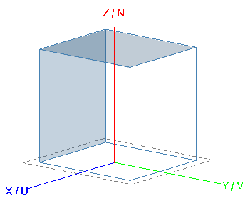
Figure 1. An example of a Cartesian boundary near field request with only the +N
surface and -V surface included (faces shown in blue).
On the Request tab, in the
Solution requests group, click the Near field icon.
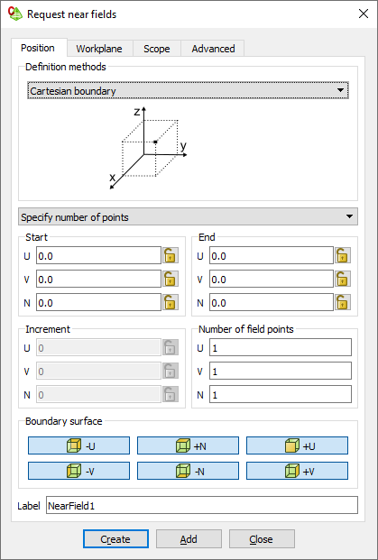
Figure 2. The Request near fields dialog.
Under Definition methods, from the drop-down list, select Cartesian
boundary.
In the drop-down list, select one of the following:
To specify the start and end points and the number of field points,
select Specify number of points.
To specify the start and end points and the increment between points,
select Specify increments.
Tip: The actual end point (depends on the start point, the
number of field points and increment) may not coincide with the
specified end point.
Under Boundary surface, clear the applicable check box
if you want to exclude a surface from the Cartesian boundary near field request.
Click on one or more of the following to exclude:
-U: Exclude the surface in the negative U
direction.
+N: Exclude the surface in the positive N
direction.
+U: Exclude the surface in the positive U
direction.
-V: Exclude the surface in the negative V
direction.
-N: Exclude the surface in the negative N
direction.
+V: Exclude the surface in the positive V
direction.
In the Label field, add a unique label for the
request.
Click Create to request the near field result and
to close the dialog.