Moving Least Squares Method (MLSM)
Builds a weighted least squares model where the weights associated with the sampling points do not remain constant.
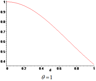
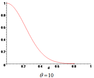
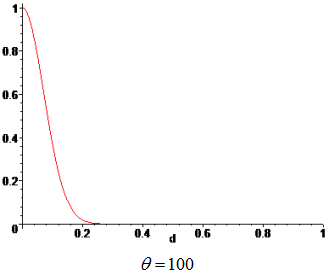
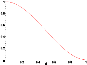
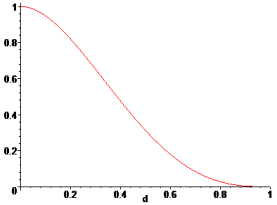
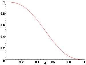
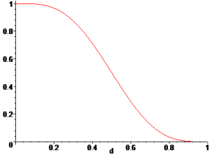
Weights are functions of the normalized distance from a sampling point to a point x, where the surrogate model is evaluated. The weight, associated to a sampling point, decays as the evaluation point moves away from it. The decay is defined through a decay function. For each point x it reconstructs a continuous function biased towards the region around that point.
Usability Characteristics
- Suggested to be used for nonlinear and noisy output responses.
- Residuals and diagnostics should be used to gain an understanding of the quality of the Fit.
- Use a Testing matrix in addition to an Input matrix for better diagnostics.
- Quality of a Moving Least Squares Method Fit is a function of the number of runs, order of the polynomial and the behavior of the application.
- If the residuals and diagnostics are not good for a Moving Least Squares Method Fit, than you can increase the order of the Fit provided you have enough runs to fit that specific order.
- Because the weights are not constant in Moving Least Squares Method, there is no analytical form and an equation can not be provided.
Settings
In the Specifications step, Settings tab, change method
settings.
Note: For most applications the default settings work optimally, and you may
only need to change the Order to improve the Fit
quality.
| Parameter | Default | Range | Description |
|---|---|---|---|
| Fit Parameter | 5.0 |
|
Controls the effect of screening out noise; the larger value, the less effect. |
| Minimum Weight | 0.001 | > 0.0 | Minimum weight. |
| Number of Excess Points | 3 | >=0 | Number of excessive points to build Moving Least Squares Method. |
| Regression Model | Linear |
|
Order of polynomial function. |
| Weighting Function | Gaussian |
|
Type of weighting function.
|