Trade Off Post Processing
Perform "What If" scenarios.
Perform "What If" Scenarios
Perform "What If" scenarios with interactive response surface tools in the Trade-Off post process tab.
- From the Post Processing step, click the Trade-Off tab.
- From the Channel selector, select the output response(s) to analyze in the Output Table.
-
Analyze the effect on inputs vs. outputs.
Option Description Modify the values of input variables to see their effect on output response approximations In the Inputs pane, change each input variable by moving the slider in the first Value column, or by entering a value into the second Value column.
Set input variables to their initial, minimum, or maximum values by moving the slider in the upper right-hand corner of the Inputs frame.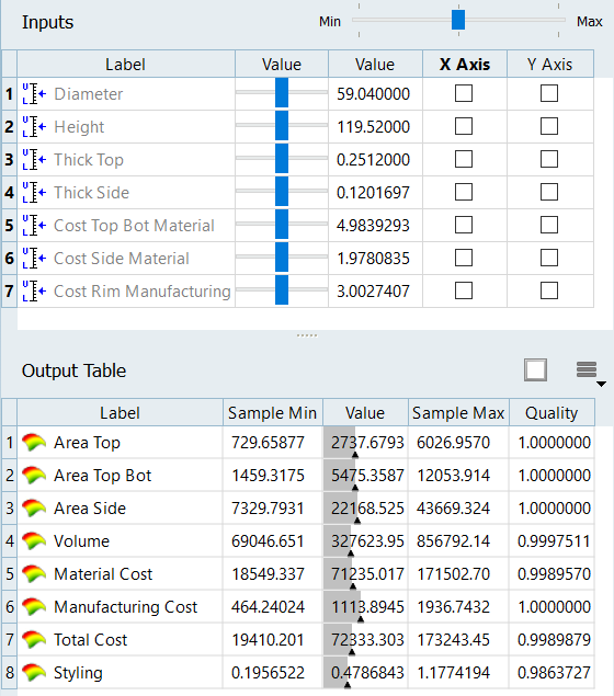
Figure 1.Plot the effect of input variables on output response approximations In the Inputs pane, select an input variable to plot by selecting its corresponding X Axis and/or Y Axis checkbox.- Create a 2D trade-off by enabling the X Axis checkbox.
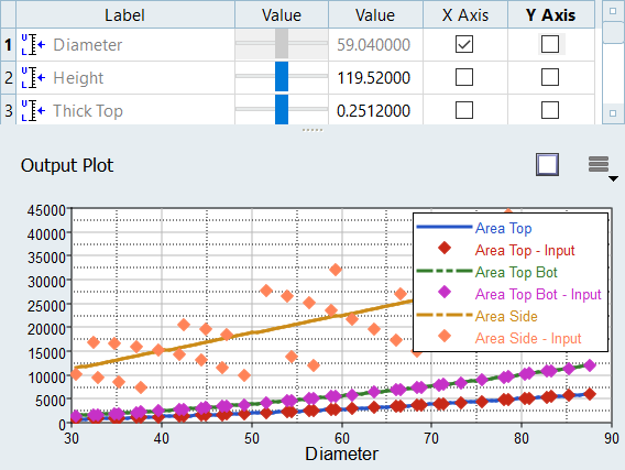
Figure 2. - Create a 3D trade off by enabling X Axis and Y Axis
checkboxes.
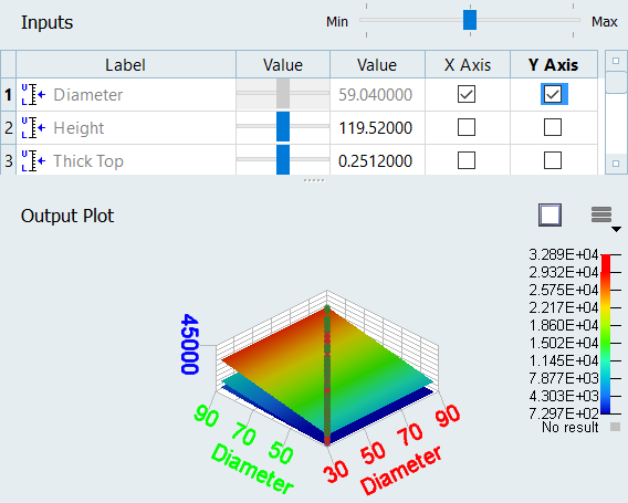
Figure 3.
The output responses selected with the Channel selector are plotted.
The values for the input variables which are not plotted can be modified by moving the sliders in the Value column to modify the other input variables, while studying the output response throughout the design space.
- Create a 2D trade-off by enabling the X Axis checkbox.
For the given values of the input variables, the output responses’ predictions are calculated by the Fit, and displayed in the Output Plot pane. Table shading is used to indicate the output response’s value between the minimum and maximum values contained in the input design matrix. When shading extends into either the Sample Min or Sample Max column, this indicates that the predicted value is beyond the bounds contained in the input matrix. If the shading extends significantly into these regions, it is suggested that you asses the validity of this value based on experience and knowledge of the modeled problem.
Trade-Off Tab Settings
Settings to configure the results displayed in the Trade-Off post processing tab.
- Fit
- Display the predicated curve (2D plot) or surface (3D plot) of the Fit.
- Fit Quality
- Plot the estimated quality (value shown in the Quality column) alongside the output response curve.
- Input Matrix
- Display the scatter points of the Input matrix.
- Testing Matrix
- Display the scatter points of the Testing matrix.
- # samples
- Change the number of discretized points used when drawing the trade-off
(2D plot) or surface (3D plot).Note: Increasing this number will result in a smoother representation, which could be at the cost of interface responsiveness.
- Discrete Surface Contour
- Display a discrete color profile of the surface. Disable this checkbox to display a blended color profile of the surface (3D plot).
- Mesh lines
- Display a visual projection of the samples' mesh grid lines onto the surface (3D plot).