HS-5010: Reliability Analysis of an Optimum
In this tutorial, you will perform a reliability analysis to determine how sensitive the objective is to small parameter variations around the optimum.
The objective has been minimized to superimpose the computed values to the reference.
In a Stochastic study, the parameters are considered to be random (uncertain) variables. This means parameters could take random values following a specific distribution (as seen in the normal distribution in Figure 1) around the optimum value (µ). The variations are sampled in the space and the designs are evaluated to gain insight into the response distribution.
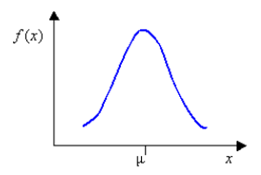
Figure 1.
Run Stochastic
In this step, you will check the reliability of the optimal solution found with GRSM. You will use Normal Distribution for the parameter variations and MELS DOE for the space sampling.
-
In the Nominal column, copy the parameter values at the optimal design.
-
Go to the Iteration History tab and copy the
optimal parameter values for R1 through AUX4 as show in Figure 2.
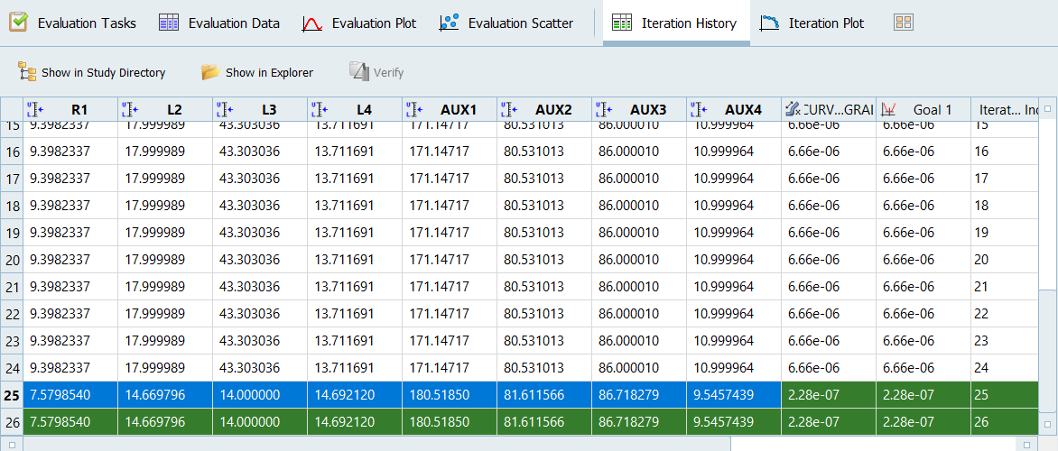
Figure 2.
-
Go to the Iteration History tab and copy the
optimal parameter values for R1 through AUX4 as show in Figure 2.
-
Go to the Bounds tab.
-
In the pop-up window, Value field, enter 0.05
and click +/-.
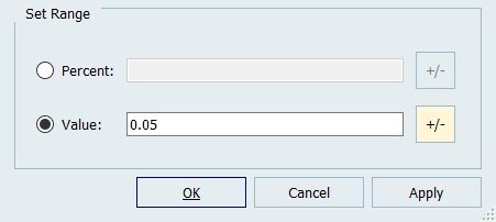
Figure 3.
The values in the 2 column (variance) of the Distributions tab are updated. -
In the pop-up window, Value field, enter 0.05
and click +/-.
Post-Process Stochastic Results
In this step, you will review the evaluation results within the Post-Processing step.
-
Go to the tab.
-
Using the Channel selector, select the
Health category to get a summarized view of
statistics and spot eventual, missing, or bad values.
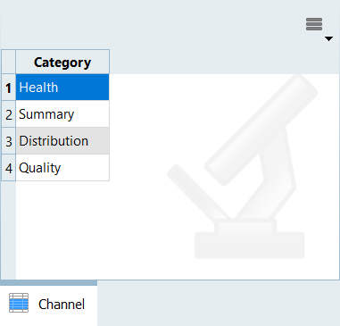
Figure 4.
-
Using the Channel selector, select the
Health category to get a summarized view of
statistics and spot eventual, missing, or bad values.
-
Review the historgrams of the Stochastic
results
-
Using the Channel selector, select
R1.
The chart in Figure 5 shows three pieces of information about the distribution of values for R1. The histogram uses the y-axis and represents the frequency of runs yielding a sub-range of response values. The probability density uses the x-axis, and indicates the relative likelihood of the variable to take a particular value. A high probability density indicates that the values are more probable to occur. The cumulative distribution uses the x-axis, and is equal to the integral of the probability density. The cumulative distribution value indicates what percentage of the data falls below the value’s threshold.
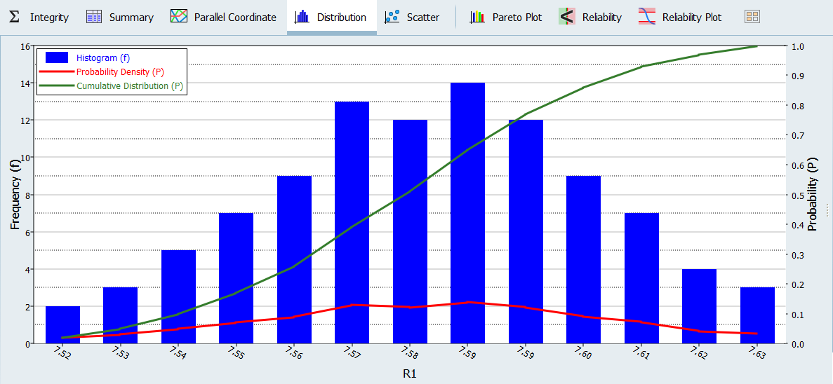
Figure 5. -
Using the Channel selector, select
CURVE_DIFF_INTEGRAL.
A high frequency of runs yields a high probability density for this response value.
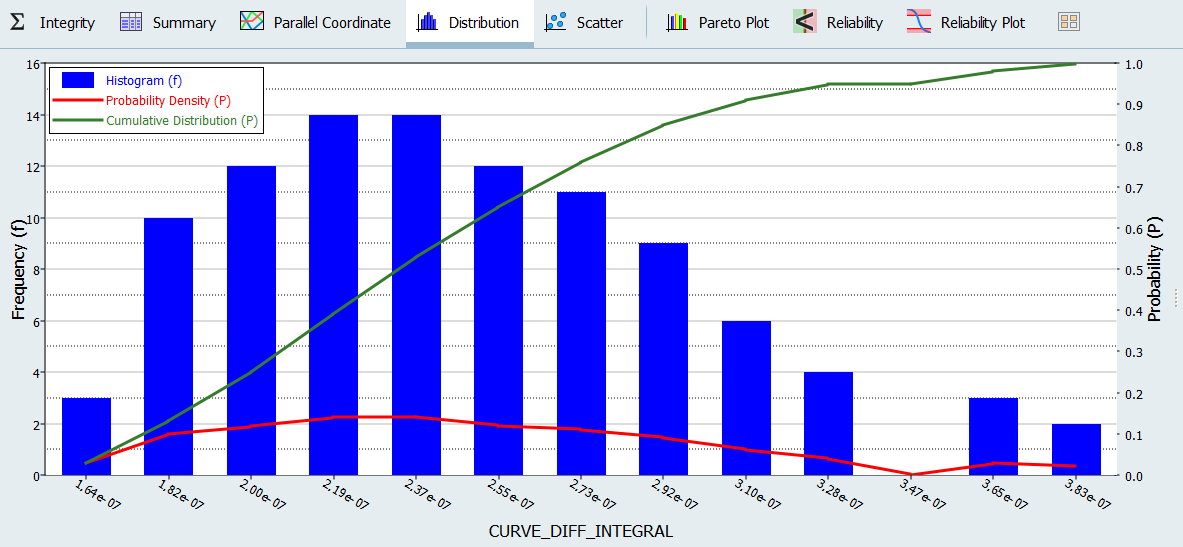
Figure 6. -
Click
 and identify the outliers identified in step 1.b.
-
Using the Channel selector, select
R1.
-
Click the Pareto Plot tab.
- From the Channel selector, select Options.
- Enable the Effect curve checkbox.
The dashed lines indicate the effect. For example, R1 has a positive effect on the response meaning the response increases higher than the optimum for R1 values. A high response value means worse matching between the computed and reference curves.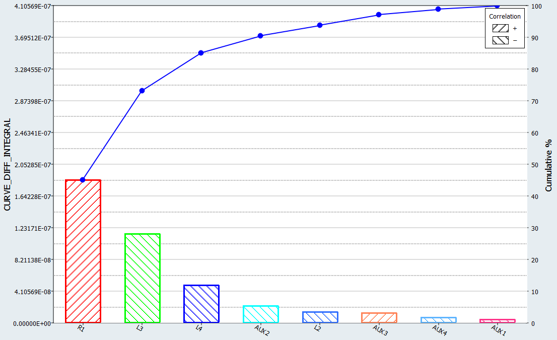
Figure 7.