HS-1630: Optimization Based on a Flux Application Example
In this tutorial, you will complete an Optimization of a die press model to get a magnet with radial orientation.
- Copy the Flux files used in this tutorial from <hst.zip>/HS-1630/ to your working directory.
- Setup Flux to work with HyperStudy. For more information, refer to the registrations steps in Flux Model.
This tutorial is based on the example TEAM 25 dedicated on the optimization of a die press model.
The figure below shows an electromagnet with the die press in the center modeled with Flux 2D. The die molds are set to form a radial flux distribution in the cavity. The objective is to get specific induction on the magnet inserted in the cavity: and along the computation path should fit the reference shown in the figure below. The table below shows the eight designs with their ranges of variation.
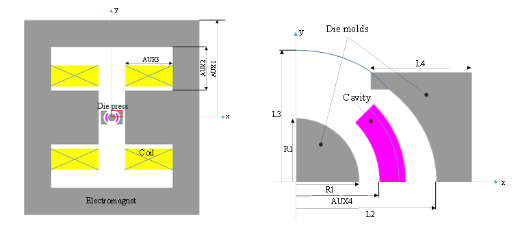
Figure 1.
| Parameter | Initial (mm) | Min (mm) | Max (mm) |
|---|---|---|---|
| R1 | 7.2 | 5 | 9.4 |
| L2 | 15.3 | 12.6 | 18 |
| L3 | 14 | 14 | 45 |
| L4 | 11.5 | 4 | 19 |
| AUX1 | 180 | 170 | 190 |
| AUX2 | 80 | 70 | 90 |
| AUX3 | 88 | 86 | 90 |
| AUX4 | 9.5 | 9.5 | 11 |
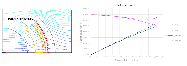
Figure 2.
Perform Study Setup
In this step, you will setup the study.
The design variables and the responses are created in Flux and are exported to HyperStudy through a link file.
-
Start a new study in the following ways:
- From the menu bar, click .
- On the ribbon, click
 .
.
-
Go to the Define Models step.
-
From the Directory, drag and drop the 4HST.F2HST
file into the work area.
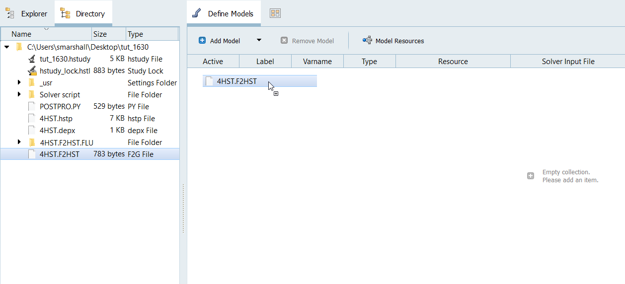
Figure 3.
HyperStudy creates a Flux model, imports eight input variables and one response from the Flux file, and populates the Solver Execution Script and Solver Input Arguments tabs. -
From the Directory, drag and drop the 4HST.F2HST
file into the work area.
-
Go to the Define Output Responses step.
-
Verify the goal is applied on Curve_DIFF_INTEGRAL
(r_1) and the type is set to
Minimize.

Figure 4.
An approach/nom_1/ directory is created inside the study directory. The directory contains the run__00001/m_1 directory where the solved Flux files are stored.
-
Verify the goal is applied on Curve_DIFF_INTEGRAL
(r_1) and the type is set to
Minimize.
Run Optimization Using GRSM
In this step, you will add and run an Optimization using the Global Response Search Method (GRSM) method.
- Optional:
Display the plots of the dvs variations vs the iterations.
-
Select Multiplot.
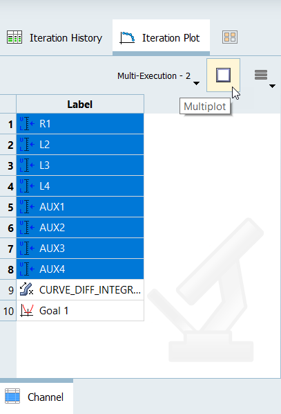
Figure 5.
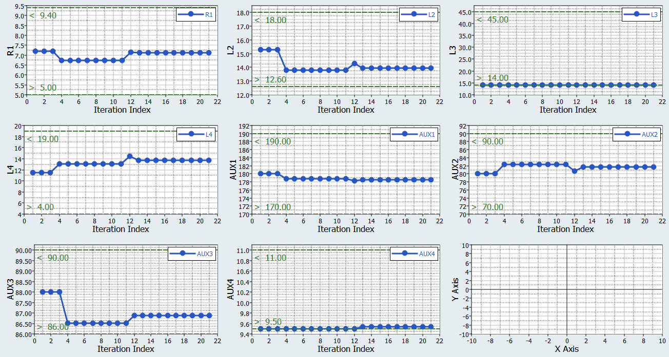
Figure 6. -
Select Multiplot.
Run Optimization Using GRSM with Inclusion Matrix
In this step, you will run a second Optimization using the Global Response Search Method (GRSM) method with Inclusion Matrix to see if a better solution can be found.
The second GRSM will start from the optimum solution found in the first Optimization ran in Run Optimization Using GRSM. The evaluations from the first Optimization using GRSM are imported as an Inclusion Matrix and 50 new runs are completed.
- From the Explorer, right-click on the GRSM Optimization approach and select Copy from the drop-down menu.
- In the Copy dialog, enter GRSM_InclMatrix for the label and click OK.
-
Go to the step.
-
For Use Inclusion Matrix, select Without Initial
from the drop-down menu to enable Use Inclusion Matrix.
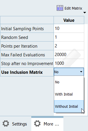
Figure 7. -
Click Edit Matrix and then select
Inclusion Matrix.
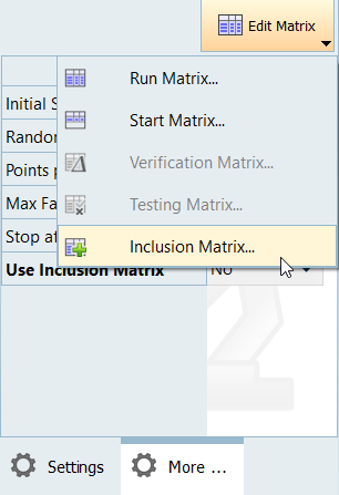
Figure 8.
-
For Use Inclusion Matrix, select Without Initial
from the drop-down menu to enable Use Inclusion Matrix.
-
Go to the Evaluate step.
Results Overview
Review the results of the tutorial.
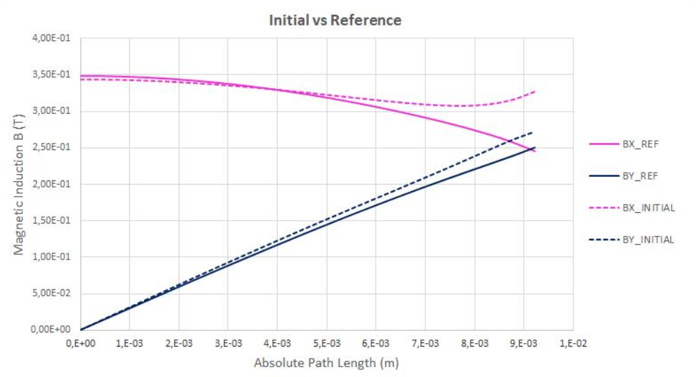
Figure 9.
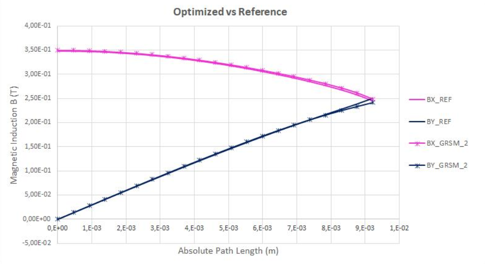
Figure 10.