HS-1540: Shape Optimization Study Using HyperMesh and ANSYS
Learn how to perform a shape Optimization started from inside HyperMesh using the direct link to HyperStudy.
Before you begin, copy the model files used in
this tutorial from <hst.zip>/HS-1540/ to your working
directory.
The finite element solver is ANSYS. HyperMorph is used to do the shape parameterization. The objective is to minimize the maximum stress of a plate with a hole. The solution can be expected to be some kind of ellipse. Hence, the input variables are the half-axes of the hole.
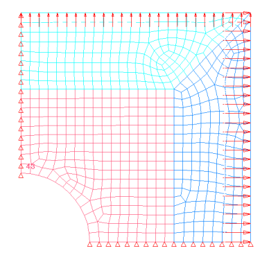
Figure 1. Double Symmetric Plate Model
Set Up Model in HyperMesh
-
Click Import.
A finite element model appears in the graphics area.
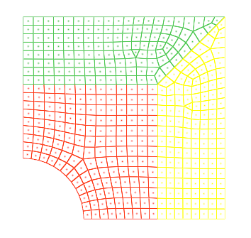
Figure 2.
Parametrize Shapes in HyperMorph
-
Generate the domains and handles that you will use to manipulate the shape of
the mesh and to generate shape perturbations for shape optimization.
- Click domains.
- Go to the create subpanel.
- Click the first arrow and select auto functions.
- Click generate.
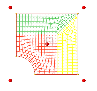
Figure 3. -
Alter dimensions.
- Go to the alter dimensions subpanel.
- Define the radius as a shape by clicking the first arrow and selecting radius.
- In the radius= field, enter 20.0000.
- Click the bottom arrow, and select hold center.
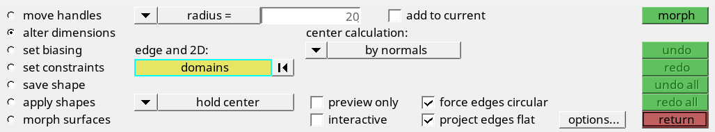
Figure 4. Settings for Alter Dimensions Subpanel -
In the graphics area, click the red edge of the hole.
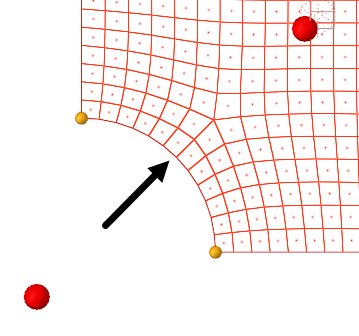
Figure 5. -
Generate second shape.
-
In the graphics area, click the lower yellow handle located in the
corner of the quarter circle.
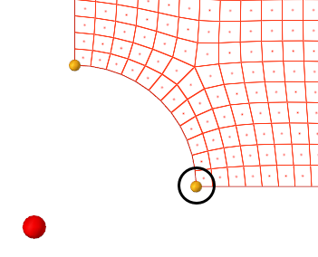
Figure 6.
-
In the graphics area, click the lower yellow handle located in the
corner of the quarter circle.
-
Generate third shape.
-
In the graphics area, click the upper yellow handle located in the
corner of the quarter circle.
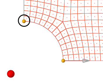
Figure 7.
-
In the graphics area, click the upper yellow handle located in the
corner of the quarter circle.
Register ANSYS as a Solver
-
Add solver script.
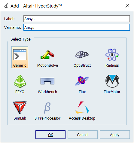
Figure 8. -
In the Path column of the script Ansys, click
 .
.
Perform the Study Setup
-
Start a new study in the following ways:
- From the menu bar, click .
- On the ribbon, click
 .
.
-
Add a HyperMesh model.
-
From the Directory, drag-and-drop the HyperMesh (.hm) file
plateDV.hm into the work area.
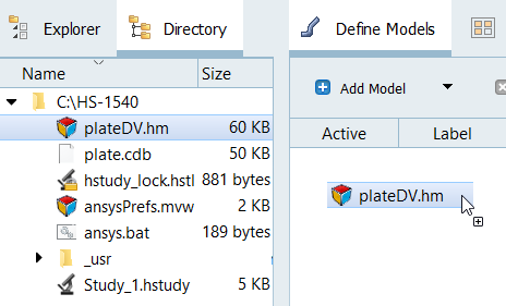
Figure 9.

Figure 10. -
From the Directory, drag-and-drop the HyperMesh (.hm) file
plateDV.hm into the work area.
-
Import variables.
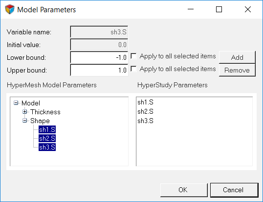
Figure 11. -
Review the input variable's lower, initial, and upper bounds.
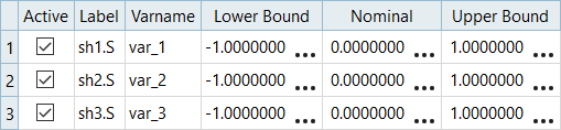
Figure 12.
Perform Nominal Run
Create and Evaluate Output Responses
Run Optimization
-
Add an objective to Response 1.
- Click Add Goal.
- In the Type column, select Minimize.

Figure 13. -
View the iteration history of the Optimization.
- Click the Iteration History tab to review the
Optimization results.
The optimal design is highlighted in green.
- Click the Iteration Plot tab to plot the Optimization results.
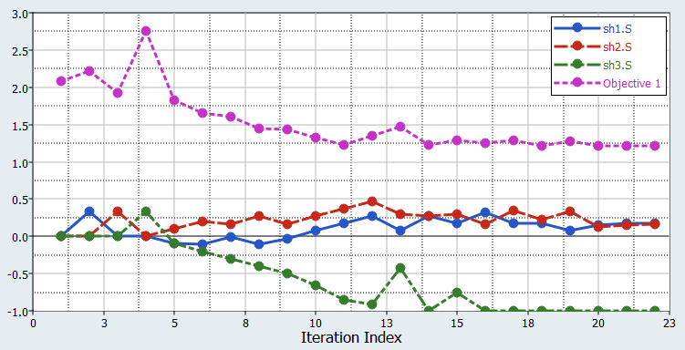
Figure 14. Iteration Plot - Click the Iteration History tab to review the
Optimization results.