OS-V: 1210 Contact with Friction

A deformable block is slid over a fixed rigid plate using enforced velocities and the problem is solved using an explicit dynamic analysis in OptiStruct. The results from OptiStruct are compared with an equivalent model in Radioss.


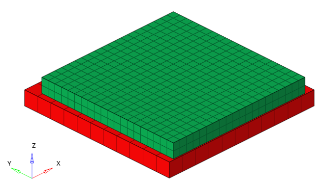
図 1. Finite Element Model

Benchmark Model

The finite element model consists of a deformable block on which enforced velocities are applied causing it to slide over a rigid fixed block.

Both blocks are meshed with first-order CHEXA elements and frictional contact is defined between the blocks with a friction coefficient = 0.05. The bottom block is constrained in all directions. One side of the top block is constrained along Y direction, while the opposite side is subjected to an enforced velocity and constrained along the X, Y, and Z rotational degrees of freedom. The upper side of the top block is subjected to an enforced velocity and is constrained along the X, Y, and Z rotational degrees of freedom.

The Y and Z directional velocities are applied in the form of a sinusoidal variation as a function of time ( t MathType@MTEF@5@5@+= feaagKart1ev2aaatCvAUfeBSjuyZL2yd9gzLbvyNv2CaerbuLwBLn hiov2DGi1BTfMBaeXatLxBI9gBaerbd9wDYLwzYbItLDharqqtubsr 4rNCHbGeaGqiVu0Je9sqqrpepC0xbbL8F4rqqrFfpeea0xe9Lq=Jc9 vqaqpepm0xbba9pwe9Q8fs0=yqaqpepae9pg0FirpepeKkFr0xfr=x fr=xb9adbaqaaeGaciGaaiaabeqaamaabaabaaGcbaGaamivaaaa@36CF@ ) given by:(1)
V = V m 2 [ 1 + sin ( 2 π T t + 3 π 2 ) ] m m / s MathType@MTEF@5@5@+= feaagKart1ev2aaatCvAUfeBSjuyZL2yd9gzLbvyNv2CaerbuLwBLn hiov2DGi1BTfMBaeXatLxBI9gBaerbd9wDYLwzYbItLDharqqtubsr 4rNCHbGeaGqiVu0Je9sqqrpepC0xbbL8F4rqqrFfpeea0xe9Lq=Jc9 vqaqpepm0xbba9pwe9Q8fs0=yqaqpepae9pg0FirpepeKkFr0xfr=x fr=xb9adbaqaaeGaciGaaiaabeqaamaabaabaaGcbaGaamOvaiabg2 da9maalaaabaGaamOvamaaBaaaleaacaWGTbaabeaaaOqaaiaaikda aaWaamWaaeaacaaIXaGaey4kaSIaci4CaiaacMgacaGGUbWaaeWaae aadaWcaaqaaiaaikdacqaHapaCaeaacaWGubaaaiaadshacqGHRaWk daWcaaqaaiaaiodacqaHapaCaeaacaaIYaaaaaGaayjkaiaawMcaaa Gaay5waiaaw2faaiaad2gacaWGTbGaai4laiaadohaaaa@4EA8@
Where, V m MathType@MTEF@5@5@+= feaagKart1ev2aaatCvAUfeBSjuyZL2yd9gzLbvyNv2CaerbuLwBLn hiov2DGi1BTfMBaeXatLxBI9gBaerbd9wDYLwzYbItLDharqqtubsr 4rNCHbGeaGqiVu0Je9sqqrpepC0xbbL8F4rqqrFfpeea0xe9Lq=Jc9 vqaqpepm0xbba9pwe9Q8fs0=yqaqpepae9pg0FirpepeKkFr0xfr=x fr=xb9adbaqaaeGaciGaaiaabeqaamaabaabaaGcbaGaamOvamaaBa aaleaacaWGTbaabeaaaaa@37EF@ and T MathType@MTEF@5@5@+= feaagKart1ev2aaatCvAUfeBSjuyZL2yd9gzLbvyNv2CaerbuLwBLn hiov2DGi1BTfMBaeXatLxBI9gBaerbd9wDYLwzYbItLDharqqtubsr 4rNCHbGeaGqiVu0Je9sqqrpepC0xbbL8F4rqqrFfpeea0xe9Lq=Jc9 vqaqpepm0xbba9pwe9Q8fs0=yqaqpepae9pg0FirpepeKkFr0xfr=x fr=xb9adbaqaaeGaciGaaiaabeqaamaabaabaaGcbaGaamivaaaa@36CF@ for Y and Z velocities are:
Direction V m MathType@MTEF@5@5@+= feaagKart1ev2aaatCvAUfeBSjuyZL2yd9gzLbvyNv2CaerbuLwBLn hiov2DGi1BTfMBaeXatLxBI9gBaerbd9wDYLwzYbItLDharqqtubsr 4rNCHbGeaGqiVu0Je9sqqrpepC0xbbL8F4rqqrFfpeea0xe9Lq=Jc9 vqaqpepm0xbba9pwe9Q8fs0=yqaqpepae9pg0FirpepeKkFr0xfr=x fr=xb9adbaqaaeGaciGaaiaabeqaamaabaabaaGcbaGaamOvamaaBa aaleaacaWGTbaabeaaaaa@37EF@ T MathType@MTEF@5@5@+= feaagKart1ev2aaatCvAUfeBSjuyZL2yd9gzLbvyNv2CaerbuLwBLn hiov2DGi1BTfMBaeXatLxBI9gBaerbd9wDYLwzYbItLDharqqtubsr 4rNCHbGeaGqiVu0Je9sqqrpepC0xbbL8F4rqqrFfpeea0xe9Lq=Jc9 vqaqpepm0xbba9pwe9Q8fs0=yqaqpepae9pg0FirpepeKkFr0xfr=x fr=xb9adbaqaaeGaciGaaiaabeqaamaabaabaaGcbaGaamivaaaa@36CF@
Y 565 mm/s 0.009 s
Z -102 mm/s 0.001 s


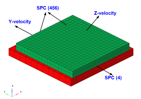
図 2. Boundary Conditions
The material properties are
Property
Value
Elastic modulus
193000 N/mm2
Poisson’s ratio
0.3
Density
7.75 E-09 tonn/mm3

Results

The Y displacement results are compared between OptiStruct and Radioss, at a node on the side, where Y-velocity is applied and they seem to be in good agreement (図 3).


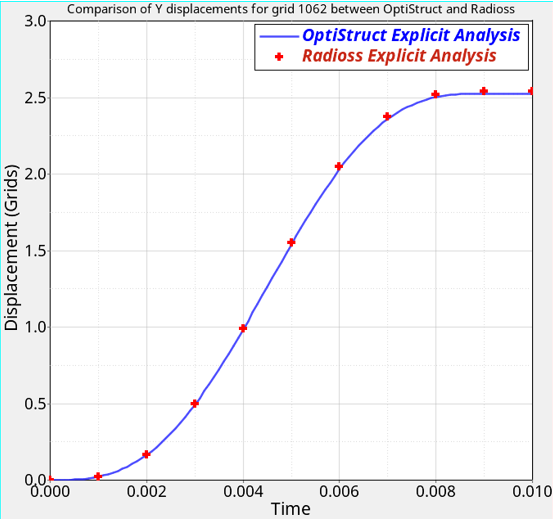
図 3. Comparison of Y displacement for a particular grid (1062)

Model Files

必要なモデルファイルのダウンロードについては、モデルファイルへのアクセスを参照してください。

The model file used in this problem includes:

contact_with_friction.fem