Rayleigh Damping (/DAMP)

In this method a proportional damping matrix is defined as:(1)

[C] = α [M] + β [K]

Where, $α$ and $β$ are the pre-defined constants. In modal analysis, the use of a proportional damping matrix allows to reduce the global equilibrium equation to n-uncoupled equations by using an orthogonal transformation.

If the global equilibrium equation is expressed as:(2)

[M] {\ddot{X}} + [C] {\dot{X}} + [K] {X} = {F_{t}}

The transformed uncoupled system of equations can be written as:(3)

{[ϕ]}^{T} [M] [ϕ] {\ddot{ξ}} + {[ϕ]}^{T} [C] [ϕ] {\dot{ξ}} + {[ϕ]}^{T} [K] [ϕ] {ξ} = {[ϕ]}^{T} {F_{T}}

With (4)

{[φ]}^{T} [C] [φ] = [\begin{matrix} α + β ω_{1}^{2} & 0 & . & . & 0 \\ 0 & α + β ω_{2}^{2} & . & . & 0 \\ . & . & . & . & . \\ . & . & . & . & . \\ 0 & . & . & . & α + β ω_{n}^{2} \end{matrix}]

Each uncoupled equation is written as:(5)

{\ddot{ξ}}_{i} + 2 ω_{i} ζ_{i} {\dot{ξ}}_{i} + ω_{i}^{2} ξ_{i} = f_{i}^{t}

With (6)

2 ζ_{i} ω_{i} = α + β ω_{i}^{2}

Where,

$ω_{i}$: The i^th natural frequency of the system
$ζ_{i}$: The i^th damping ratio

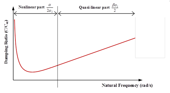
This leads to a system of

n

equations with two unknown variables

α

and

β

. Regarding to the range of the dominant frequencies of system, two frequencies are chosen. Using the pair of the most significant frequencies, two equations with two unknown variables can be resolved to obtain values for

α

and

β

. For high frequencies the role of

β

is more significant. However, for lower frequencies

α

plays an important role (図 1).

The Rayleigh damping method applied to explicit time-integration method leads to the following equations:(7)

M γ^{t} + C v^{t} = F_{e x t}^{t} - F_{int}^{t}

With

C = α M + β K

(8)

F_{int}^{t} = F_{int}^{t - d t} + K v^{t - \frac{d t}{2}} d t

(9)

v^{t} = v^{t - \frac{d t}{2}} + γ^{t} \frac{d t}{2}

(10)

M γ_{0}^{t} = F_{e x t}^{t} - F_{int}^{t}

Neglecting

F_{e x t}^{t} - F_{e x t}^{t - d t}

and

v^{t} - v^{t - \frac{d t}{2}}

, in

β K v^{t}

evaluation you have:(11)

K v^{t} = K v^{t - \frac{d t}{2}} = \frac{F_{int}^{t} - F_{int}^{t - d t}}{d t} \approx M \frac{(γ_{0}^{t} - γ_{0}^{t - d t})}{d t}

And finally:(12)

γ_{0}^{t} = M^{- 1} (F_{e x t}^{t} - F_{int}^{t})

(13)

γ^{t} = \frac{γ_{0} - α v^{t - \frac{d t}{2}} - \frac{β}{d t} (γ_{0}^{t} - γ_{0}^{t - d t})}{1 + α \frac{d t}{2}}

(14)

v^{t + \frac{d t}{2}} = v^{t - \frac{d t}{2}} + γ^{t} d t

The three approaches available in Radioss are Dynamic Relaxation (/DYREL), Energy Discrete Relaxation (/KEREL) and Rayleigh Damping (/DAMP). Refer to Example Guide for application examples.

The loading is applied at a rate sufficiently slow to minimize the dynamic effects. The final solution is obtained by smoothing the curves.

In case of elasto-plastic problems, one must minimize dynamic overshooting because of the irreversibility of the plastic flow.