Example 7: 16x16 Short Dipole Array with Binomial Algorithm
This case explains how to use the binomial algorithms to calculates the pointing parameters in a bidimensional short dipole array.
Step 1 Create a new MoM Project.
Open newFASANT and select File - New option.
Figure 1. New Project panel
Select MOM option on the previous figure and start to configure the project.
Step 2 Set the simulation parameters as shown.
Select Simulation - Parameters option, set the parameters and save it.
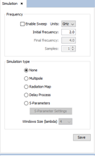
Figure 2. Simulation panel
Step 3 Create the array.
Click on Source - Dipole - Dipole Array to create an array of 16x16 electrical short dipoles, with a spacing of 0.04 m, that are oriented following the y-axis. The array is located on the XY plane. The spacing of 0.04m is equivalent to a spacing of 0.267 in units of lambda, at a frequency of 2 GHz.
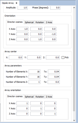
Figure 3. Dipole Array panel
Step 4 Feed the array.
To set the feeding of the array select Source - Antenna Feeding and the following panel will open.
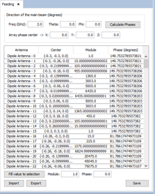
Figure 4. Antenna Feeding panel
This is the default setting. To use the binomial algorithm click on Tools - User Function and select the corresponding function. NOTE: To use the bidimensional binomial function it is needed to download both the bidimensional and the unidimensional functions.
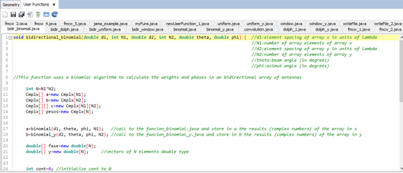
Figure 5. Bidimensional Uniform function
A path has been selected by default so the files will be created on the mydatafiles folder in the newFASANT directory.
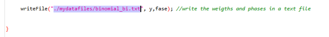
Figure 6. Bidimensional Uniform function
The next step is generating the text file. To do so click on Tools - Calculator and write the call to the function.
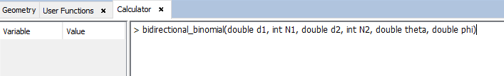
Figure 7. Calculator panel
- d1: element spacing of the array in the x axis in units of lambda
- N1: number of array elements of the array in the x axis
- d2: element spacing of the array in the y axis in units of lambda
- N2: number of array elements of the array in the y axis
- theta: beam angle, in degrees
- phi: azimuth angle, in degrees
In this case, set the parameters as shown. Angles of theta=45º and phi=0º are selected as an example.
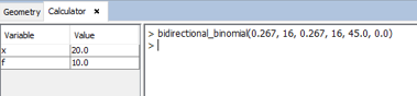
Figure 8. The text file will be automatically generated in the mydatafiles folder.
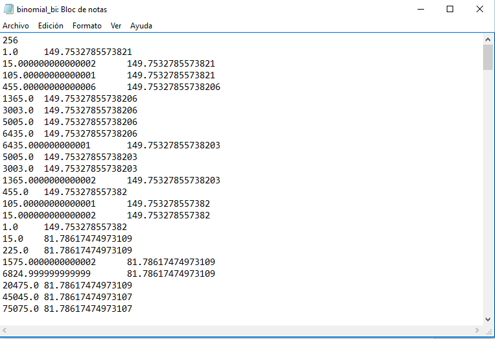
Figure 9. Results file
Now, apply these results to the array created before by clicking on S ource - Antenna Feeding.
The panel shown before will appear. To use the weights and phases calculated with the binomial algorithm, click on Import.
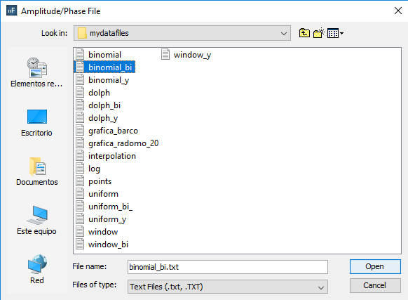
Figure 10. Amplitude/Phase File panel
Select the corresponding file and save the feeding.
Step 5 Create ground plane.
In order to avoid unwanted radiation to go below the array, create a ground plane using the plane command, or Geometry - Surface - Plane. The array is situated in the XY plane with z=0, so the z coordinate has to be negative.

Figure 11. Plane parameters
View of the dipole array.
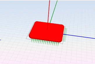
Figure 12. Array view
Step 6 Solver parameters.
Select Solver - Advanced Options and set the parameters as shown.
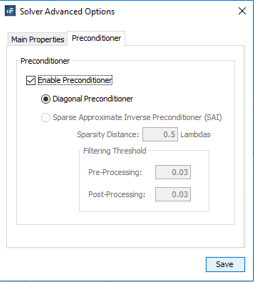
Figure 13. Solver Advanced Options panel
Step 7 Meshing the geometry model.
Select Mesh - Create Mesh to open the meshing configuration panel and then set the parameters as show the next figure.
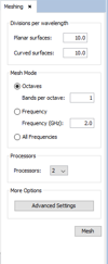
Figure 14. Meshing panel
Click on Mesh.
Step 8 Execute the simulation.
Select Calculate - Execute option to open simulation panel.
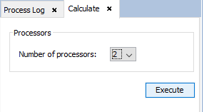
Figure 15. Calculate panel
Step 9 Show Results.
The radiation cuts can be visualized by clicking on Show Results - Radiation Pattern - View Cuts.
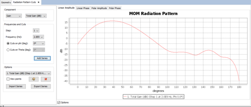
Figure 16. Radiation Pattern Cuts
The radiation pattern can be visualized by clicking on Show Results - Radiation Pattern - View 3D Pattern.
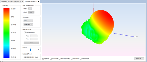
Figure 17. Radiation Pattern 3D
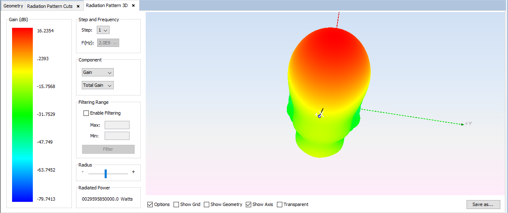
Figure 18. Radiation Pattern 3D