Scatter in Fatigue Material Data

Handle scatter in fatigue test results.

The SN and EN curves (and other fatigue properties) of a material are obtained from experiment, through fully reversed rotating bending tests. 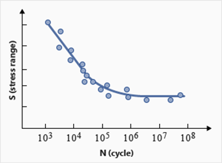Due to the large amount of scatter that usually accompanies test results, statistical characterization of the data should also be provided (certainty of survival is used to estimate the worst mean log(N) according to the standard error of the curve and a higher reliability level requires a larger certainty of survival).

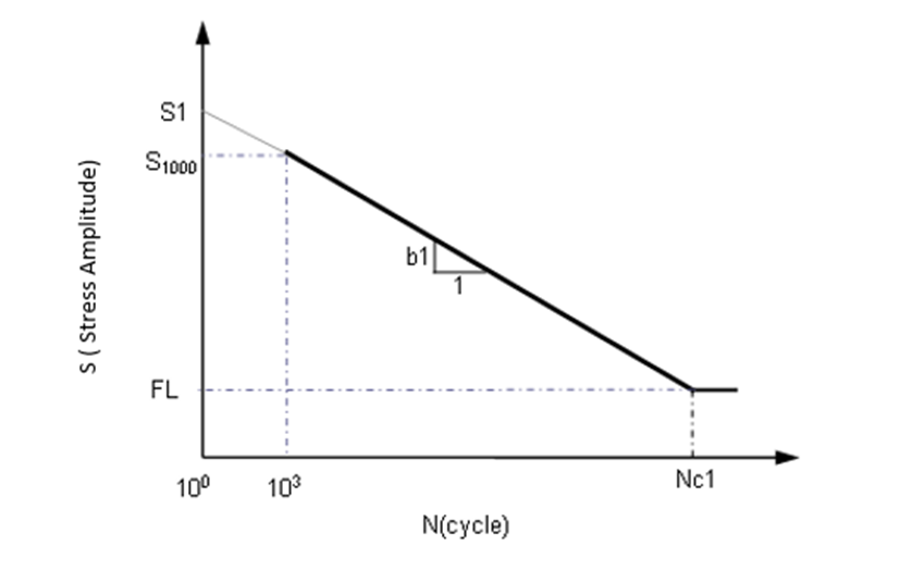
To understand these parameters, consider the SN curve as an example. When SN testing data is presented in a log-log plot of alternating nominal stress amplitude S_a or range S_R versus cycles to failure N, the relationship between S and N can be described by straight line segments. Normally, a one or two segment idealization is used.

Consider the situation where SN scatter leads to variations in the possible SN curves for the same material and same sample specimen. Due to natural variations, the results for full reversed rotating bending tests typically lead to variations in data points for both Stress Amplitude (S) and Life (N). Looking at the Log scale, there are variations in Log(S) and Log(N). Specifically, looking at the variation in life for the same Stress Amplitude applied, a set of data points may look like this:

S	Log (S)	Log (N)
2000.0	3.3	3.9
2000.0	3.3	3.7
2000.0	3.3	3.75
2000.0	3.3	3.79
2000.0	3.3	3.87
2000.0	3.3	3.9

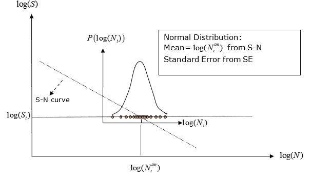
As with many processes, the distribution of Log(N) is assumed to be a Normal Distribution. There is a full population of possible values of log(N) for a particular value of log(S). The mean of this full population set is the true population mean and is unknown. Therefore you statistically estimate the worst true population mean of log(N) based on your input sample mean (SN curve) and Standard Error (SE) of your sample. The SN material data input is based on the mean of the normal distribution of the scatter in the particular sample used to generate the data.

The experimental scatter exists in both Stress Amplitude and Life data. The Standard Error of the scatter of log(N) is required as input (SE field for SN curve). The sample mean is provided by the SN curve as $\log (N_{i}^{s m})$ whereas, the standard error is input via the SE field.

If the specified SN curve is directly utilized, without any perturbation, then the sample mean is directly used, leading to a certainty of survival of 50%. This implies that you do not perturb the sample mean you provided. Since a value of 50% survival certainty may not be sufficient for all applications, SimSolid can internally perturb the SN material data to the required certainty of survival defined by you. To accomplish this, the following data is required:

Standard error of log(N) normal distribution SE
Certainty of Survival required for this analysis

A normal distribution or gaussian distribution is a probability density function which implies that the total area under the curve is always equal to 1.0.

The SN curve data you defined is assumed as a normal distribution, which is typically characterized by the following Probability Density Function:(1)

P (x_{s}) = \frac{1}{\sqrt{2 π σ_{s}^{2}}} e^{- \frac{{(x_{s} - μ_{s})}^{2}}{2 σ_{s}^{2}}}

Where:

$x_{s}$ is the data value ( $\log (N_{i})$ ) in the sample you defined.

$μ_{s}$ is the sample mean ( $\log (N_{i}^{s m})$ ).

$σ_{s}$ is the standard deviation of the sample (which is unknown, as you input only Standard Error (SE).

The above distribution is the distribution of the sample you defined, and not the full population space. Since the true population mean is unknown, the range of the true population mean is estimated from the sample mean and the sample SE, and then the Certainty of Survival you defined is used to perturb the sample mean.

Standard Error is the standard deviation of the normal distribution created by all the sample means of samples drawn from the full population. From a single sample distribution data, the Standard Error is typically estimated as $S E = (\frac{σ_{s}}{\sqrt{n_{s}}})$ , where $σ_{s}$ is the standard deviation of the sample, and $n_{s}$ is the number of data values in the sample. The mean of this distribution of all the sample means is actually the same as the true population mean. The certainty of survival you provided is applied on this distribution of all the sample means.

Generally, you convert a normal distribution function into a standard normal distribution curve (which is a normal distribution with mean = 0.0 and standard error = 1.0). You can then directly use the certainty of survival values via Z-tables.

Note: The certainty of survival is equal to the area of the curve under a probability density function between the required sample points of interest. It is possible to calculate the area of the normal distribution curve directly (without transformation to standard normal curve), however, this is computationally intensive compared to a standard lookup Z-table. Therefore, you generally first convert the current normal distribution to a standard normal distribution and then use Z-tables to parametrize the input survival certainty.

For the normal distribution of all the sample means, the mean of this distribution is the same as the true population mean $μ$ , the range of which is what you want to estimate.

Statistically, you can estimate the range of true population mean as follows:

(2)

\log (N_{i}^{s m}) - z * S E \leq μ \leq \log (N_{i}^{s m}) + z * S E

That is,

(3)

\log (N_{i}^{s m}) - z * S E \leq \log (N_{i}^{m}) \leq \log (N_{i}^{s m}) + z * S E

Since the value on the left side is more conservative, use the following equation to perturb the SN curve:

(4)

\log (N_{i}^{m}) = \log (N_{i}^{s m}) - z * S E

Where,

$\log (N_{i}^{m})$ is the perturbed value

$\log (N_{i}^{s m})$ is the sample mean you defined (SN curve)

$S E$ is the standard error (SE)

The value of

z

is procured from the standard normal distribution Z-tables based on the input value of the certainty of survival. Some typical values of Z for the corresponding certainty of survival values are illustrated in the table below.

Z-values (calculated)	Certainty of Survival (Input)
0.0	50.0
-0.5	69.0
-1.0	84.0
-1.5	93.0
-2.0	97.7
-3.0	99.9

Notice how the SN curve is modified to the required certainty of survival and standard error input. This technique allows you to handle fatigue material data scatter using statistical methods and predict data for the required survival probability values.