Post Processing
Learn to automatically post-process results from ultraFluidX using the template automation tool HWGenImages.
Methods and Process
This program directs AcuFieldView, running in batch, to read in simulation data and write out specified images and plots. These plots and images can also be written to a PDF and/or PPT or plot data exported to a text file. The images and views described below use a subset of available tools in HWGenImages and have been selected specifically for small SUV/Sedan automobile aerodynamics. A complete list of options is available in HWGenImages documentation.
Live interactive sessions to visualize ultraFluidX results can be opened manually in AcuFieldView as part of the AcuSolve software package. When opening ultraFluidX results with AcuFieldView, the .layout file will open the partitioned mesh results in parallel and the .bcf file will open the combined results in serial if available. Files are also provided by ultraFluidX for Paraview. The .sos file will open the partitioned mesh results in parallel and the .case file will open the combined results in serial if available.
The images, views and ranges shown in this section are the current best practices of presenting the data, identified by interviewing industry experts, online resources and literature.
Assumptions
- All quantities used are averaged in time over in the converged flow regime
- Yaw, roll and steer angle are 0
- Pressure is converted into the Coefficient of Pressure to normalize the quantity such that different speeds show the same force
Template
- General
- The following can be modified for all images:
- Background color
- Outline of image on or off
- Font size
- Font
- Variables
- Many of the quantities used in the template are based on the model size
and simulation setup. The defaults used in the general template are for
a midsize SUV, the Altair Arc. The variables are listed below and should
be updated as needed:
meanVel = inflow speed
resultsDir = path to results directory
carLength = length of automobile
carWidth = width of automobile
carHeight = height of automobile
dx = intervals to move the coordinate surface by in the x direction
dy = intervals to move the coordinate surface by in the y direction
dz = intervals to move the coordinate surface by in the z direction
- Cover Sheet
- Contains a user specified title and picture. The image must be generated
during the template automation. The images is then identified to be on
the cover page.
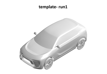
Figure 1. - Run Summary
- The run summary from ultraFluidX is
displayed here as a reference. You can omitt this if desired.
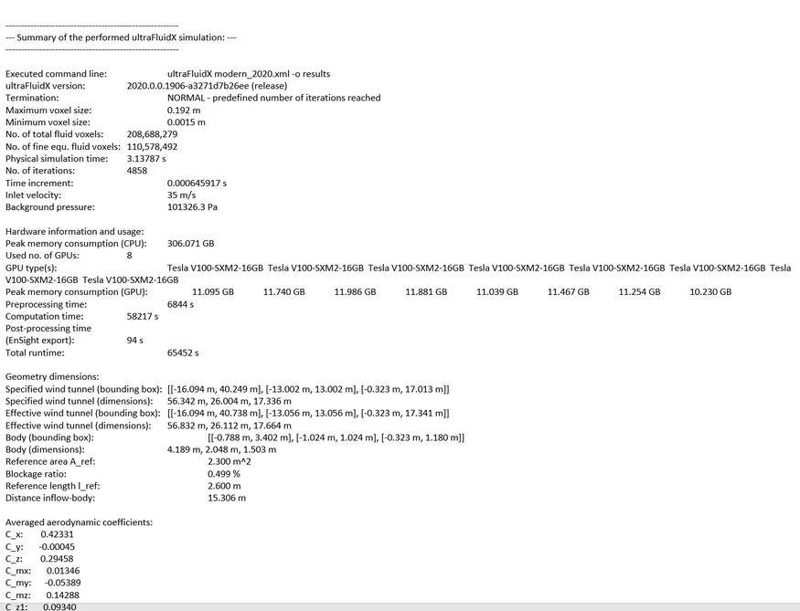
Figure 2. - Cumulative Lift/Drag Plot
- Averaged cumulative averaged lift and drag are plotted along to
automobile. This plot illustrates how the drag and lift progress along
the vehicle. Areas with high contributions can be identified so they
explored further. The cumulative quantity is computed at each section
(the number of sections are identified in the uFX input file) and summed
with the sections prior, moving from front to rear. The last value is
the averaged lift and drag quantity for the vehicle.
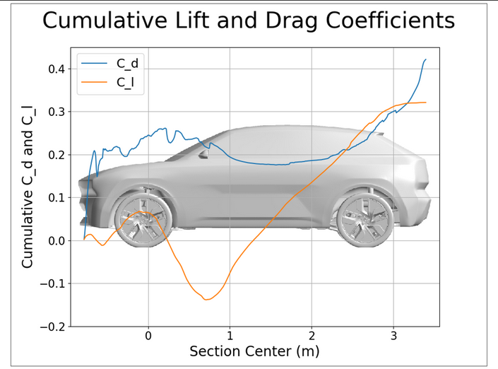 Figure 3. Cumulative Sectional C_d and C_l with background
image
Figure 3. Cumulative Sectional C_d and C_l with background
image - Sectional Drag and Lift Plot - in X Direction
-
The sectional lift and drag from from front to rear is plotted next. This shows where the greatest contribution of lift and drag are along the car. These are only in 2D, so the forces in each section are summed together and displayed. The number of sections here are taken for the value set in uFX input file.
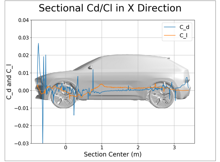
Figure 4. X Sectional C_d and C_l with background image - Instantaneous Lift and Drag Progression
- Monitoring the convergence history shows how the quantities of lift and
drag progressed through time. If these quantities are still changing
significantly (steady increase or decrease) at the end of the simulation
time, then the simulation time should be increased to ensure a stable
region is within the averaging window.
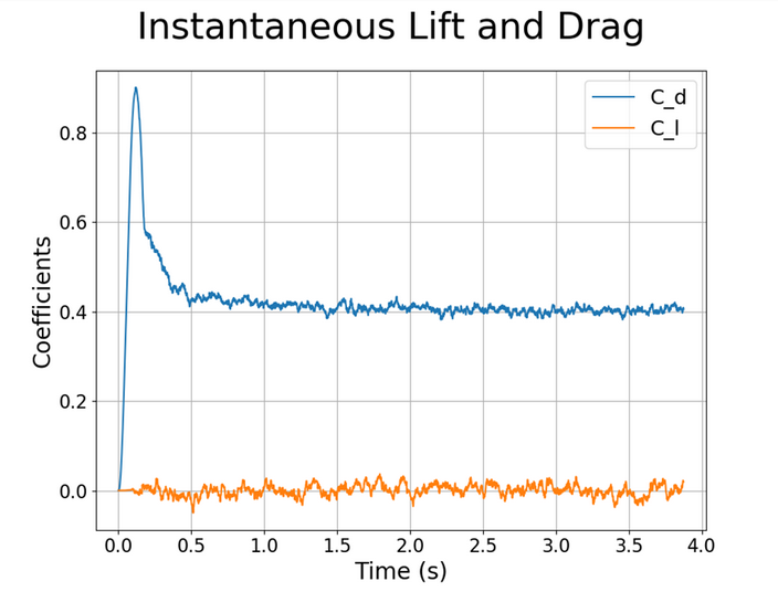
Figure 5. - Heat Exchange Mass Flow Rate Plot
- The mass flow through the heat exchangers are plotted next. These values
are shown over time as to monitor how the simulation progresses in
computing them. The units are (kg/sec).
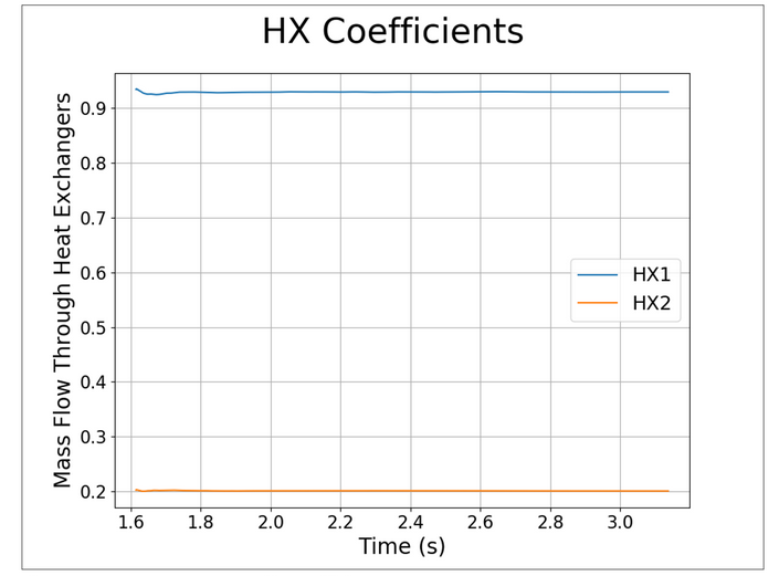
Figure 6. Average porous media coefficients - Component Level Lift/Drag
- Component lift and drag help in identifying the largest contributors of lift and drag for the automobile.
- Automobile Surface Images
- Images from automobile are included from multiple angles to show users
what the overall model looks like. The views should be sufficient to
show large design changes.
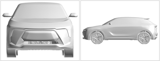
Figure 7.A specific area can be identified as an area of interest.
- Pressure Images
- Visualizing pressure on the surface communicates where there is a high
force (red) from the air pushing on the car and low force (blue) from
suction. The pressure force is converted to the Coefficient of Pressure
and displayed from multiple angles. The fast transition from red to blue
indicates a separation region which greatly influences the performance
of the vehicle.
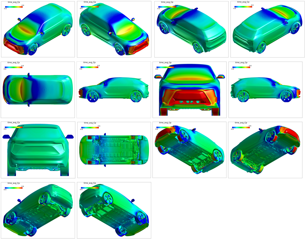
Figure 8.The rear vehicle has low pressure due to separation at the C pillars. To visualize the pressure in the rear more efficiently, adjust the range down. Here a range of Cp -0.3 to 0 is used.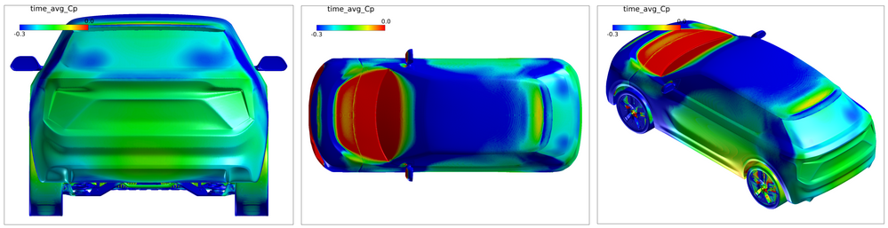
Figure 9. - Coefficient of Friction Images
-
Coefficient of friction is a measure of the resistance that a surface exerts on a substance moving over it; in this case, air moving over the vehicle. An area with a high Cf value (red) indicates air moving at a high velocity close to the body. Low (blue) Cf indicates lower speed regions and in some cases separated flow. Separation is observed when the quantity of Cf changes drastically on a part of the body. For example, a change of red to blue on the hood indicates that the flow was moving fast on the surface but then separated due to adverse pressure gradient in the boundary layer and is no longer attached. Separation on the front of the vehicle generally increases drag.
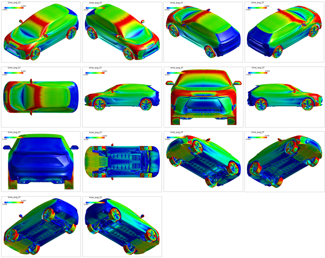
Figure 10. - ISO Surface Images
-
ISO surface of several quantities are the next set of images to be displayed. An ISO surface is a surface in the fluid volume defined by a specified value of the identified quantity. These surface aid in visualizing the flow structures in the fluid volume, not constrained by model definition.
The first ISO surface is of the Coefficient of Pressure Total with a value of 0. This ISO surface is colored by the scalar- time averaged velocity magnitude m/s. The shape and size of the surface shows where CpT=0 is located, thereby showing where pressure is lower than the Total Pressure. These regions are of particular interest as they identify where the pressure differential is pulling the vehicle, or drag. The coloring of the ISO surface highlights regions with quickly moving fluid near low CPT zones, indicating a region of separation.
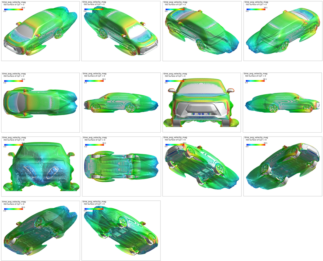
Figure 11.The next ISO surface is of X velocity equal to 0 m/s, colored by the scalar- time averaged Coefficient of Pressure. This ISO surface communicates where the air has stopped moving despite the car moving. These are areas of completely detached, recirculating flow.
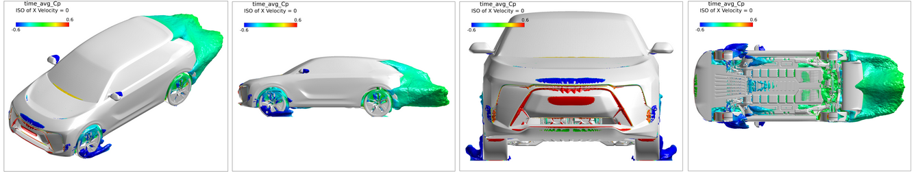
Figure 12. - Slice Plane Images
- Interrogating the flow field with slice planes identifies what is
happening in the air surrounding the vehicle. First you view slice planes in the X direction of time averaged velocity magnitude in increments of 0.1m, viewed from the front then from the rear.
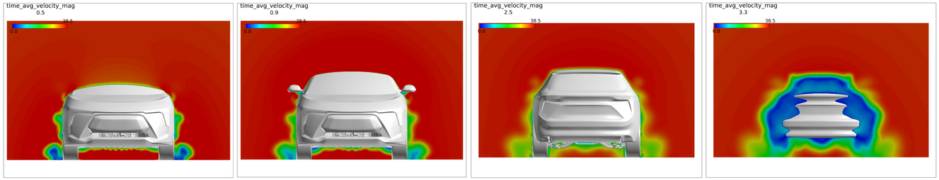
Figure 13. -
Next, focus on the flow under the hood, again viewing time averaged velocity magnitude, but this time trim the vehicle so you can view the under hood region.
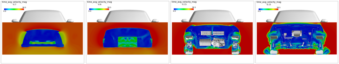
Figure 14.Then use the y plane to view the velocity in the wake. These slice planes are taken at a specified interval of 0.1 m. Moving through the planes provides insight on the wake size and shape.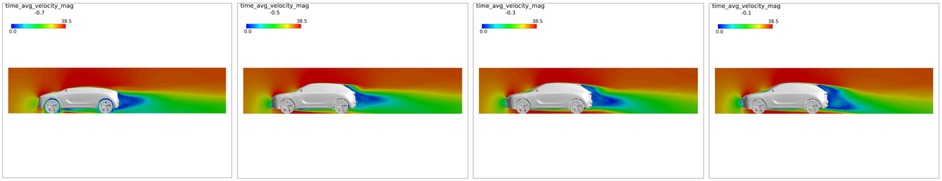
Figure 15.Lastly, velocity magnitude is viewed from the Z plane starting at the floor looking towards the vehicle, then from above the vehicle. The plane moves at increments of a specified value of 0.1m from the ground to above the vehicle.
Here grid lines are displayed in the plane as well as the velocity magnitude. This is helpful when viewing multiple design iterations to identify the changes in the wake.
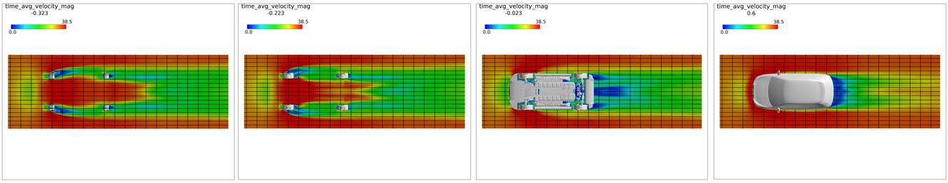
Figure 16.Resolution setup for various types of vehicles in ultraFluidX. These Best Practices have been derived using Industry standard/public models, as well as client project experience. Best practices are reviewed and improved with each release. For an overview on ultraFluidX and the requirements needed to run the solver, please refer to the Altair ultraFluidX 2020 User Guide.