Troubleshoot
Learn troubleshooting techniques for common simulation issues.
The simulation of a model is the third phase of a three-phased process. The evaluation and compilation phases occur first generating a structure that is used during the simulation phase of the software. Some error-handling techniques can help with issues that may occur during these phases.
Evaluation Errors
- Uninitialized Variables
-
Block parameter values are defined in terms of OML expressions. These expressions may contain OML variables. Activate uses specific scoping rules for the evaluation phase: In general a variable can be used in a block expression if it has been defined in the context of a diagram containing the block, or in the initialization script. Variables used in the diagram contexts must also be defined following the scoping rules. Note in particular that variables defined in the OML base workspace are not systematically added to the model workspace.
If the evaluation phase finds an uninitialized variable, then the variable should be defined in the proper context or in the initialization script. Note that all the variables used within a masked super block must be defined within the super block, either as a mask parameter or in a context.
If variables are used in the definition of the simulation parameters associated with the model but not a specific diagram, then these variables must be defined in the initialization script.
- Inconsistent Parameter Types
-
Block parameter expressions are evaluated and checked against the type of constraints imposed by the block. For example if a parameter accepts only a numerical matrix for value, but the evaluation of its expression leads to a string, then an error is generated.
Compilation Errors
The main role of the compilation phase is to find the simulation function associated with every block, and to construct scheduling tables specifying the order in which the block simulation functions must be called during a simulation. Common errors encountered at this stage include algebraic loops and incompatible data types and sizes.
- Algebraic Loops
-
An algebraic loop occurs if block activations in a model cannot be scheduled for simulation. For example, a block A can be activated to produce its outputs only if the values of block A’s inputs are already available from the blocks producing the inputs by way of a feedthrough property. This scenario implies that block A must be scheduled after the scheduling of the blocks producing the inputs. Therefore, if a model contains a path going through the input ports of blocks containing feedthrough properties, and the path loops back through the model, then every block in the loop requires the value of its output to compute its output, which is of course a contradiction. In this case no scheduling can be performed and the model is said to have an algebraic loop. Generally, such loops do not occur in a correctly-formulated model. If the model is sound, the presence of loops may be due to an erroneous feedthrough property setting in a user-defined block. If the loop does occur in a correctly-formulated model, incorporating a LoopBreaker block into the model can break the loop.
Algebraic loops may involve activation signals. For example the output of an integrator with a jump option is synchronized with the event causing the jump so that the output cannot be used to define the new state of the integrator. The problem is that the output at activation time is the value after the jump so the output depends on the new value of the state. In general, the user intent is that the value of the new state be computed based on the value of the output just before the jump, and not after. A solution is to add a LastInput block to the model. This block provides the left limit of its input signal, therefore if the integrator output goes through this block to define the new state, the activation at the jump time provides the desired value for the new state and the loop is broken.
An algebraic loop can occur when a super block is made atomic. This operation may introduce additional artificial feedthrough properties resulting in algebraic loops in a model which was previously loop free.
- Incompatible Port Data Types and Sizes
-
The compilation phase determines the data types and sizes of the signals that connect blocks via regular ports. Most blocks in the software accept different data types and sizes of signals but may impose certain constraints. The connections impose additional constraints, in particular that the data type and size of the connected ports be identical, with the exception that a real output port can be connected to a complex port. A role of the compilation is to find the data types and sizes of all the connecting signals in order to satisfy the constraints.
In some cases, the constraints imposed on the signal data types and sizes are inconsistent and the fixed-point iteration strategy implemented by the compiler to determine the data types and sizes fails for the following reasons:
- Row or Column Vector Distinction
-
Signals in the software are matrices with two dimensions. A scalar signal is a 1x1 matrix. Strictly speaking, a vector signal data type does not exist; but a vector is often considered to be an nx1 matrix, such as a column vector. Using a row vector instead of a column vector can raise size inconsistency errors in some blocks.
- Data Type Propagation
-
Most blocks impose their inputs and outputs to have similar data types. For example the Sum block accepts all Activate data types (real, complex, various integers) but all inputs and the output must have the same data type. For this reason, the data type often gets propagated throughout a model. If signals of different data types are required in a model, then the adding of a DatatypeConversion block may be required to explicitly perform the casting from one data type to another.
- Imposing Data Type and Size Constraints on New Blocks
-
When creating a new block, a custom block or a library block, allowing inputs and outputs of different data types and sizes is useful, if possible. A sophisticated mechanism is in play to specify general constraints on port data types and sizes, but in most cases, constraints can be imposed by using negative numbers to specify an unknown size or data type. For example if the size of an input is defined as [-1,1], then the input can have any number of rows but only one column. If the same block has another input of size [-2,-1] then this input has as many columns as the first input had rows and any number of rows. Thus, a negative value used in the definition of a port size implies a free value, but the same negative value used in the definition of another port size of the same block implies that the two sizes have the same value. The same applies to data types.
Simulation Performance
Simulation performance generally depends on the model complexity and required precision of the simulation. In some cases, however, the simulation time may be significantly reduced by bringing small modifications to the model.
- OML Custom Blocks
-
OML custom blocks provide options to define block simulation behavior with OML. OML programs are easy to develop and debug, moreover they enable access to all of the functions available in OML libraries. But OML is an interpreted language and its performance is significantly poorer than compiled languages such as C. As a result, continuously activated OML custom blocks can significantly reduce simulation performance.
If simulation time becomes an issue, OML blocks should be replaced with Activate basic blocks, in particular Math and Matrix Expression blocks, or the C custom block. OML custom blocks that are only activated at discrete times usually do not degrade significantly the performance of models that include continuous-time dynamics.
- Zero Crossings
-
Variable-step solvers modify their steps-sizes during simulation. To satisfy the imposed error tolerances, the solvers take smaller steps when required, but go back to taking larger steps when possible reducing the simulation time. The fundamental assumption when using a variable step solver is that the dynamical system being solved is smooth, in general at least twice differentiable.
If the model being simulated is not smooth, which is generally true with hybrid systems, then the time interval must be divided into distinct intervals such that over each interval a smooth dynamical system is exposed to the numerical solver. If not, the solver may have to reduce significantly its step-size to go beyond a non-smooth point; it may even fail.
The software includes a sophisticated mechanism for implementing this strategy based on distinguishing critical events from non-critical events. Critical events are used to specify max step-sizes and cold-restart actions during the simulation.
The software’s compiler and simulator identify and manage most critical events, but when a non-smooth source is inside of a block, then that source must be exposed by the block itself. This is done in particular by declaring zero-crossing surfaces. Most non-smooth blocks in the installed library declare zero-crossings, but they also provide the option to turn off zero-crossings. Particular situations can occur where using a zero-crossing mechanism creates out of range signals causing solver failure. In such situations, the zero-crossing option of a block must be turned off; otherwise zero-crossing options must be turned on for all blocks to achieve good simulation performance.
For the same reason, all user-defined blocks containing non-smooth dynamics, Custom blocks or not, must implement a zero-crossing surface if they are to be activated in continuous-time.
- Solver Choice
-
The software provides a number of numerical solvers. Some solvers may be better adapted to some models. There is no simple rule for choosing the right solver but in general a variable-step solver should be used if possible, unless there is a specific reason for using a fixed-step solver. If the variable-step solver fails or is too slow, even after relaxing error tolerances, something that happens in general when the model contains hidden non-smoothness, then fixed-step solvers can be used. The choice of the step size should be made appropriately. Note that fixed-step solvers do not have any error control mechanism.
- Sliding Mode
-
Hybrid systems can switch from one dynamics to another during simulation. In some cases the time differences from one switching to the next may go to zero (Zeno behavior) with the solution converging to a surface. It is possible to reformulate the dynamics of the system to obtain its behavior constrained to this sliding surface. The dynamics is then said to be in sliding mode. But such a transformation cannot be done by a general purpose solver such as Activate. If the sliding surfaces are declared properly with zero-crossings then the solver stops and restarts at each switching time, assuming a variable-step solver is used, and so the simulation ends up freezing at some point.
If the sliding surface is not implemented with zero-crossings, the simulation may proceed slowly and the solution exhibits high frequency chattering. This may provide an acceptable approximate solution to the original model with sliding mode. Using a fixed-step solver may be an alternative in this case. But in most cases, if the sliding mode is really present in the model and is not the result of a modeling error, then modifications to the model should be considered. This may include introducing additional dynamics, hysteresis or explicit time delays to reduce the chattering. Such behaviors generally better represent the actual dynamics of control models where a sliding mode is encountered.
- Scope and Display Blocks
-
Excessive use of Scope and Display blocks can slow down a simulation. A large number of such blocks can be present in a model for debugging purposes, but only a few are truly needed for a given simulation run. To improve simulation time, you can turn off the status for some of these blocks. Turning off the status removes the blocks from the simulation structure and changes the simulation performance to be identical to that of having completely removed the blocks.
- Real Time Scaling
-
The model parameter for Real Time Scaling slows down a simulation so that it can run in real time. A slow simulation may happen if this parameter is not set correctly. Setting the parameter value to zero makes the simulation run as fast as possible.
- Profiling
- You can generate a .csv profiling file
(<modelname>_profile.csv) that contains valuable information
for analyzing your simulation. From the ribbon, select .
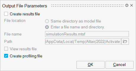
When you run a simulation, in addition to the results file, a profiling file, <modelname>_profile.csv, is generated and stored in the temporary directory (tempdir) for the model.Note: The tempdir is displayed in the OML Command window when you run a simulation. You can query the location of the directory with the command: GetCurrentModelTempDir.The profiling file includes the execution time of each block and the number of times and conditions (flags) under which the block is called during the simulation. The information is displayed in columns for each block and provides the number of times a block is called for each flag. The flags are defined as follows:
Flag Number Issued Flag Definition Flag 0 VssFlag_Derivatives Flag 1 VssFlag_OutputUpdate Flag 2 VssFlag_StateUpdate Flag 3 VssFlag_EventScheduling Flag 4 VssFlag_Initialize Flag 5 VssFlag_Terminate Flag 6 VssFlag_Reinitialize Flag 7 VssFlag_ReinitializeImplicit Flag 8 VssFlag_Projection Flag 9 VssFlag_ZeroCrossings Flag 10 VssFlag_Jacobians Flag 11 VssFlag_GotoPause Flag 12 VssFlag_ReturnFromPause
Simulation Failures
- Singularity in a Block
-
If a block simulation function performs a computation with inputs that are out of range, for example, by a division by zero, then an error is generated. The acceptable operations may depend on the supported data types. For example, the Log block does not accept negative real inputs because its output is defined to be real; the Log block does accept negative inputs of a complex data type.
Note: Singularity problems may be encountered at the start of a simulation when all the block outputs by default are set to zero. - Frozen Simulation
-
The presence of sliding mode may cause slow simulation but in some cases may halt the simulation or generate an error. See Sliding Mode for more details.
- Non-Convergence
-
The non-convergence of a solver is in general due to the presence of an unstable mode in the model. The divergence may occur very rapidly but in general can be confirmed by adding Scope blocks to the model for visualizing the values of the states. Another possible reason for non-convergence is the presence of hidden non-smoothness.
Error Messages
- Unsupported Visual C++ Target Option
- During some use cases, for example, simulation of Modelica models or FMI import or export, the software issues an error if unable to detect a C++ compiler installed on the system. To correct the error, install a supported Microsoft Visual Studio C++ compiler. To view the compiler installed on your system, from the OML command window, enter vssGetCompilerName().