nyquist
Nyquist diagram.
Syntax
nyquist(sys)
nyquist(sys, w)
nyquist(..., fmt, ...)
nyquist(..., property, value, ...)
[re, im, w] = nyquist(...)
Inputs
- sys
- A linear time-invariant transfer function or state space system.
- w
- The vector of frequencies at which to compute the response. The units are radians/sec for continuous time, and Hz for discrete time. If w is a two-element vector, it contains the range of frequencies over which to compute the response. The units are radians/sec for continuous time, and Hz for discrete time.
- fmt
- Plot format arguments. See the plot function help.
- property
- Plot property arguments that are paired with a following value. See the plot function help.
- value
- Plot property value arguments. See the plot function help.
Outputs
- re
- The real component of the response.
- im
- The imaginary component of the response.
- w
- The vector of frequencies at which to compute the response. The units are radians/sec for continuous time, and Hz for discrete time.
Example
Create the Nyquist diagram of the given 3rd order analog transfer function, with the plot in red.
tfo = tf([1,1,3,3],[1,-3,3,-1]);
nyquist(tfo,'r');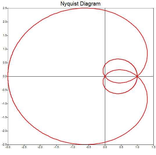
Figure 1. nyquist figure 1
Comments
If the output arguments are omitted, the function plots the results.
If w is omitted, then internally computed values are used.
By default, 500 points are plotted. More points can be requested using the w input, in which case it is typically best to specify them with logspace.
nyquist does not currently provide special treatment for sys inputs with poles or zeros on the imaginary axis.
nyquist does not currently support MIMO systems.