ACU-T: 3200 Radiation Heat Transfer in a Simple Headlamp using the Enclosure Radiation Model

Prerequisites

This tutorial introduces you to setting up a radiation heat transfer problem using the Enclosure radiation model in HyperMesh and solving using AcuSolve. Prior to starting this tutorial, you should have already run through the introductory HyperWorks tutorial, ACU-T: 1000 HyperWorks UI Introduction, and have a basic understanding of HyperMesh, AcuSolve, and HyperView. To run this simulation, you will need access to a licensed version of HyperMesh and AcuSolve.

Before you begin, copy the file(s) used in this tutorial to your working directory.

Since the HyperMesh database (.hm file) contains meshed geometry, this tutorial does not include steps related to geometry import and mesh generation.

Problem Description

The problem to be solved is shown schematically in Figure 1 and Figure 2. It consists of a simple headlamp with a housing, lens, and a bulb. The inner cavity of the bulb is filled with air and the wattage of the bulb is 1W, which is modeled as a volumetric heat source. The Boussinesq density model is used for the air to consider the natural convection effects in the fluid volume. The heat generated in the bulb is transferred by three means: conduction from the bulb to the housing, natural convection in the air volume, and radiation from the bulb surface to other surfaces. The external reference temperature is 300 K for the outer surfaces of the headlamp. You will use the Enclosure radiation model to simulate the surface to surface radiation.


Figure 1.
The enclosure radiation methodology in AcuSolve involves a two-step process: view factor computation and heat flux addition. View factor is the proportion of radiation incident one surface due to another surface. The view factors are computed, and the radiative heat fluxes are added to the energy equation during the solver run. These radiative heat fluxes are computed based on the view factors using the Stefan-Boltzmann law. The enclosure radiation model is supported only on fluid mediums.


Figure 2.

Open the HyperMesh Model Database

  1. Start HyperMesh Desktop and load the AcuSolve user profile.
    Refer to the HM introductory tutorial, ACU-T: 1000 HyperWorks UI Introduction, to learn how to select AcuSolve from User Profiles.
  2. Click the Open Model icon located on the standard toolbar.
    The Open Model dialog opens.
  3. Browse to the directory where you saved the model file. Select the HyperMesh file ACU-T3200_HeadlampEnclosure.hm and click Open.
  4. Click File > Save As.
    The Save Model As dialog opens.
  5. Create a new directory named Headlamp_Enclosure and navigate into this directory.
    This will be the working directory and all the files related to the simulation will be stored in this location.
  6. Enter Headlamp_Enclosure as the file name for the database, or choose any name of your preference.
  7. Click Save to create the database.

Set the General Simulation Parameters

Set the Analysis Parameters

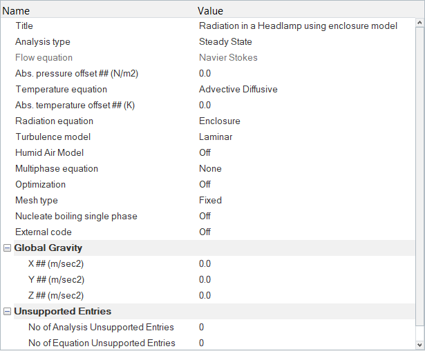
  1. Go to the Solver Browser, expand 01.Global, then click PROBLEM_DESCRIPTION.
  2. In the Entity Editor, verify that the Analysis type is set to Steady State.
  3. Set the Temperature equation to Advective Diffusive.
  4. Set the Radiation equation to Enclosure.
  5. Set the Turbulence model to Laminar (if not set already).


    Figure 3.

Specify the Solver Settings

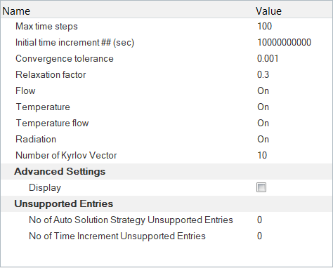
  1. In the Solver Browser, click 02.SOLVER_SETTINGS under 01.Global.
  2. In the Entity Editor, turn On Temperature flow.
  3. Leave the remaining options unchanged.


    Figure 4.

Define the Material Models and the Body Force

Define the Material Models

  1. In the Solver Browser, expand 02.Materials > Fluid then click on Air_HM.
  2. In the Entity Editor, change the Density type to Boussinesq.
  3. In the Solver Browser, under 02.Materials, right-click on SOLID and select Create.
  4. In the Entity Editor, name it Arnite.
  5. Set the Density to 1670 kg/m3.
  6. Set the Specific heat to 2050 J/kg-K.
  7. Set the Conductivity to 1.65 W/m-K.
  8. Repeat steps 3-7 and create two more solid material models, Plastic and LED, with the following material properties:
    1. Plastic:
      1. Density - 1270 kg/m3
      2. Specific heat - 1900 J/kg-K
      3. Conductivity to 0.22 W/m-K
    2. LED:
      1. Density - 5500 kg/m3
      2. Specific heat - 0.3 J/kg-K
      3. Conductivity to 5.0 W/m-K
  9. Save the database.

Define the Body Force

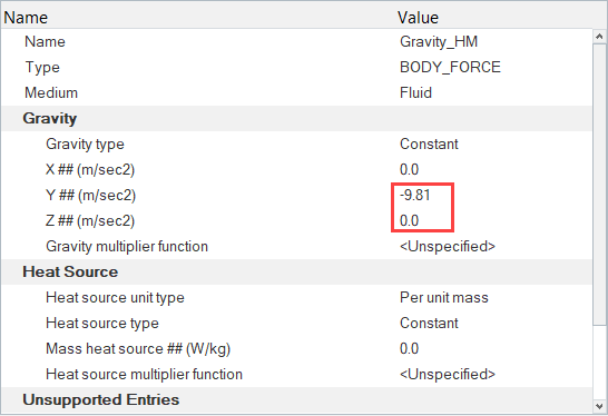
  1. In the Solver Browser, expand 03.Body_Force > BODY_FORCE then click on Gravity_HM.
  2. In the Entity Editor, set the Y-Gravity to -9.81 m/sec2 and change to Z-Gravity to 0.


    Figure 5.

Define the Heat Source

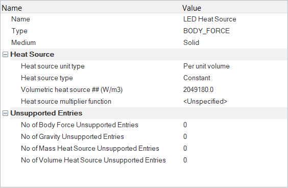
  1. In the Solver Browser, right-click on 03.Body_Force and select Create.
  2. In the Entity Editor, name it LED Heat Source.
  3. Change the Medium to Solid.
  4. Set the Heat source unit type to Per unit volume.
  5. Set the Heat Source type to Constant and set the Volumetric heat source to 2049180 W/m3.


    Figure 6.

Set the Boundary Conditions

Create the Emissivity Model

  1. In the Solver Browser, right-click on 07.Emissivity_Model and select Create.
  2. In the Entity Editor, name it Walls.
  3. Set the Emissivity to 0.7.

Set the Boundary Conditions

By default, all components are assigned to the wall boundary condition. In this step, you will change them to the appropriate boundary conditions and assign material properties to the fluid volumes.
  1. In the Solver Browser, expand 12.Surfaces > WALL.
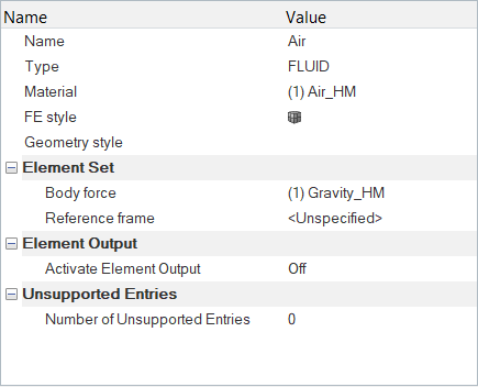
  2. Click Air. In the Entity Editor,
    1. Change the Type to FLUID.
    2. Set the Material to Air_HM.
    3. Set the Body force to Gravity_HM.


    Figure 7.
  3. Click Housing. In the Entity Editor,
    1. Change the Type to SOLID.
    2. Set the Material to Plastic.


    Figure 8.
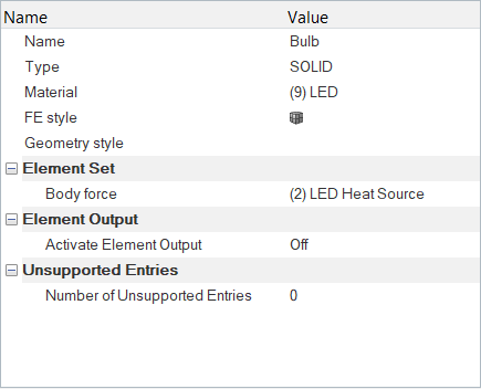
  4. Click Bulb. In the Entity Editor,
    1. Change the Type to SOLID.
    2. Set the Material to LED.
    3. Set the Body force to LED Heat Source.


    Figure 9.
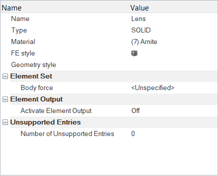
  5. Click Lens. In the Entity Editor,
    1. Change the Type to SOLID.
    2. Set the Material to Arnite.


    Figure 10.
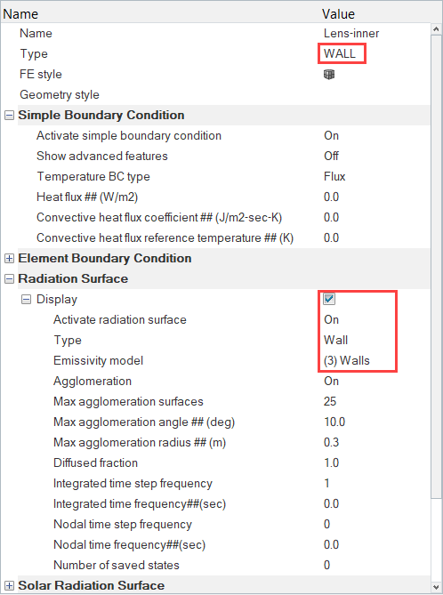
  6. Click Lens-inner. In the Entity Editor,
    1. Verify that the Type is set to WALL.
    2. Under the Radiation Surface tab, activate the Display checkbox, set the Activate radiation surface field to On, set the Type to Wall, and set the Emissivity model to Walls.


    Figure 11.
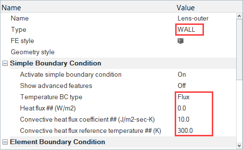
  7. Click Lens-outer. In the Entity Editor,
    1. Verify that the Type is set to WALL and the Temperature BC type is set to Flux.
    2. Set the Convective heat flux coefficient to 10 J/m2-sec-K.
    3. Set the Convective heat flux reference temperature to 300 K.


    Figure 12.
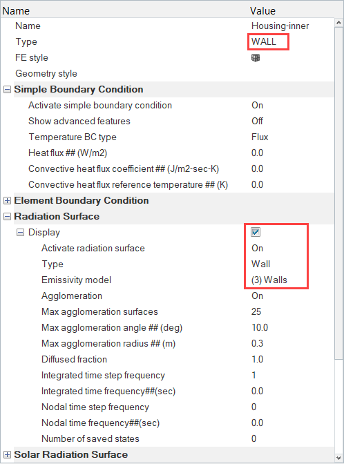
  8. Click Housing-inner. In the Entity Editor,
    1. Verify that the Type is set to WALL.
    2. Under the Radiation Surface tab, activate the Display checkbox, set the Activate radiation surface field to On, set the Type to Wall, and set the Emissivity model to Walls.


    Figure 13.
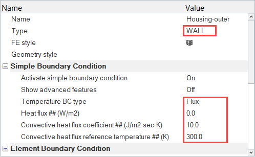
  9. Click Housing-outer. In the Entity Editor,
    1. Verify that the Type is set to WALL and the Temperature BC type is set to Flux.
    2. Set the Convective heat flux coefficient to 10 J/m2-sec-K.
    3. Set the Convective heat flux reference temperature to 300 K.


    Figure 14.
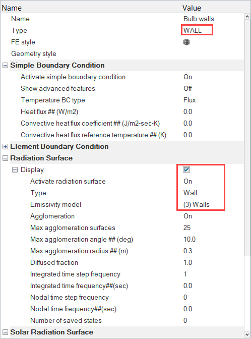
  10. Click Bulb-walls. In the Entity Editor,
    1. Verify that the Type is set to WALL.
    2. Under the Radiation Surface tab, activate the Display checkbox, set the Activate radiation surface field to On, set the Type to Wall, and set the Emissivity model to Walls.


    Figure 15.
  11. Save the model.

Run AcuSolve

In this step, you will launch AcuSolve to compute a solution for this case.

  1. Turn on the visibility of all mesh components.
    For the analysis to run, the mesh for all active components must be visible.
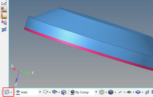
  2. Click on the ACU toolbar.
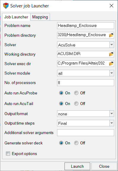
    The Solver job Launcher dialog opens.
  3. Optional: For a faster solution time, set the number of processors to a higher number (4 or 8) based on availability.
  4. Leave the remaining options as default and click Launch to start the solution process.


    Figure 16.

Post-Process the Results with HyperView

In this step, you will visualize the results using HyperView. While doing so, you will create contour plots of temperature and velocity magnitude on a section cut and also create a plot of velocity vectors. Once the solver run is complete, close the AcuProbe and AcuTail windows. In the HyperMesh Desktop window, close the AcuSolve Control tab and save the model.

Switch to the HyperView Interface and Load the AcuSolve Model and Results

  1. In the HyperMesh Desktop window, click the ClientSelector drop-down in the bottom-left corner of the graphics window.


    Figure 17.
  2. Select HyperView from the list.
  3. In the pop-up dialog that appears, click Yes.
    The interface is changed to HyperView.

    Once HyperView is loaded, the Load model and results panel should be open by default. If you do not see the panel, click File > Open > Model.

  4. In the Load model and results panel, click next to Load model.
  5. In the Load Model File dialog, navigate to your working directory and select the AcuSolve .Log file for the solution run that you want to post-process. In this example, the file to be selected is Headlamp_Enclosure.1.Log.
  6. Click Open.
  7. Click Apply in the panel area to load the model and results.
    The model is colored by geometry after loading.

Create a Contour Plot of Temperature

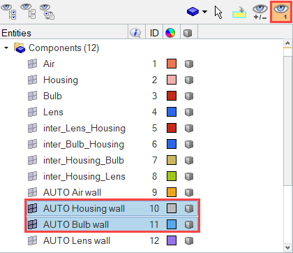
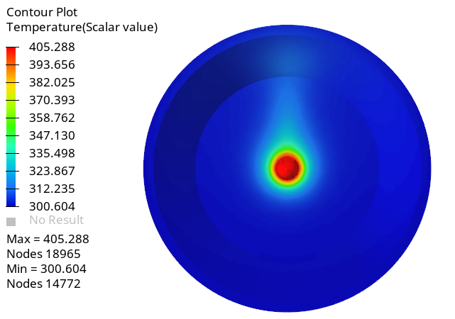
  1. In the Results Browser, expand the list of Components then click the Isolate Shown icon .
  2. Hold Ctrl and select the AUTO Housing wall and AUTO Bulb wall components to turn off the display of all the components except the walls of the bulb and housing components.


    Figure 18.
  3. Orient the display to the xy-plane by clicking on the Standard Views toolbar.
  4. Click on the Results toolbar to open the Contour panel.
  5. In the panel area, set the Result type to Temperature (s).
  6. Click the Components entity selector. In the Extended Entity Selection dialog, select Displayed.
  7. Click Apply.
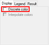
  8. In the panel area, under the Display tab, turn off the Discrete color option.


    Figure 19.
  9. Click the Legend tab then click Edit Legend. In the dialog, change the Numeric format to Fixed then click OK.


    Figure 20.

Display Temperature Contours and Velocity Vectors on a Section Cut

In this step, you will create a section cut on the mid-z plane and then display the temperature and velocity vectors on that cross section.

  1. In the Results Browser, turn on the display of all the components.
  2. Click the Section cut icon icon on the HV-Display toolbar.
  3. In the panel area, click Add to create a new section cut named Section 1.
  4. In the Define plane section, set the axis to Z Axis then click Apply.
  5. Set the Z base coordinate to 0.0005 then press Enter.
  6. Change the Display options from Clipping plane to Cross section.


    Figure 21.
  7. Click Gridline. In the Gridline Options dialog, deactivate the Show check box under Grid line then click OK.
  8. Click the Vector icon on the Results toolbar to open the Vector panel.
  9. In the panel area, set the Result type to Velocity (v).
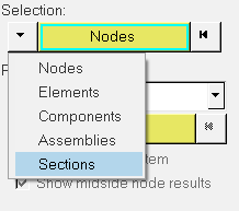
  10. Click the Selection drop-down and select Sections from the list of options.


    Figure 22.
  11. Click the Sections entity selector then select All.
  12. In the panel area, activate the Overlay result display check box (if not set already).
  13. Click Apply.
  14. Under the Plot tab, verify that only the X+Y+Z Resultant option is selected.
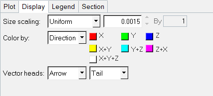
  15. Go to the Display tab, set the Size scaling option to Uniform, and enter a value of 0.0015 in the size field.
  16. Set the Color by option to Direction and set the X+Y+Z color to White.


    Figure 23.
  17. Go to the Section tab, activate the Projected check box, then click Apply.
  18. Click on the Results toolbar to open the Contour panel.
  19. In the panel area, set the Result type to Temperature (s).
  20. Click the Components entity selector. In the Extended Entity Selection dialog, select Displayed.
  21. In the panel area, under the Result tab, activate the Overlay result display check box (if not set already).


    Figure 24.
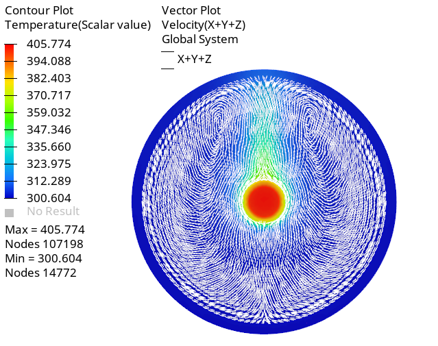
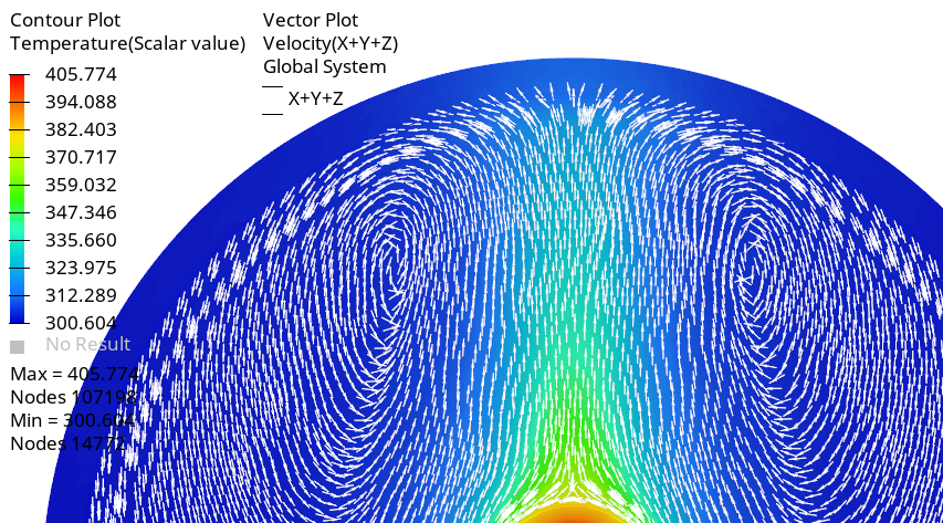
  22. Click Apply to create the contour plot of temperature on the section cut along with velocity vectors.


    Figure 25.
    Zoom in to the contour plot to observe the natural convection phenomenon inside the headlamp.


    Figure 26.

Summary

In this tutorial, you learned how to set up and solve a radiation heat transfer problem in a headlamp using the enclosure radiation model in AcuSolve. You started by importing the HyperMesh database with the mesh and basic model organization and then set up the simulation parameters and boundary conditions. Once the solution was computed, you processed the results using HyperView, where you created contour plots of temperature and velocity vectors in the fluid domain.