Analysis Tasks - General Entities
-
Click .
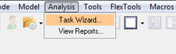
Figure 1.The Task Wizard – Component Analysis window opens.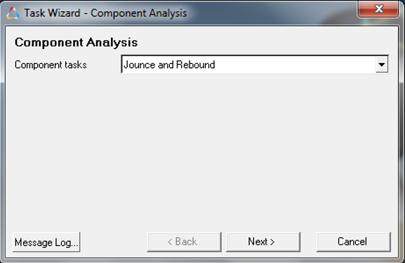
Figure 2. -
Now you have selected the required analysis data for the model, click
Finish button to complete the process and exit Task
Wizard.
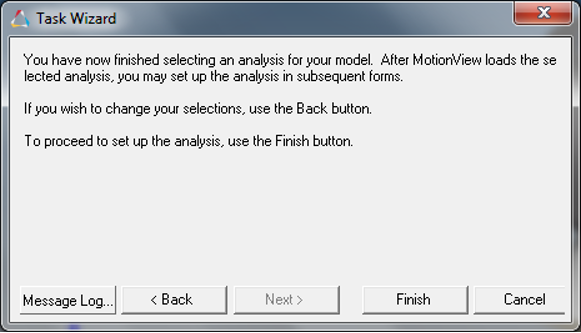
Figure 3. -
Select the required options in the Test Rig settings section.
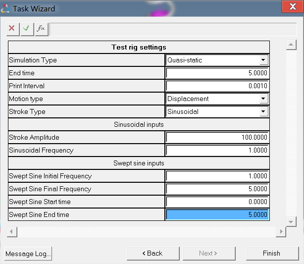
Figure 4. -
Select Transient or Quasi-Static
option from the Simulation Type drop-down menu and select the
sinusoidal or swept-sinusoidal
option from the Stroke Type drop-down list and enter the required values in the
Sinusoidal inputs and Swept sine inputs sections, then click
Finish.
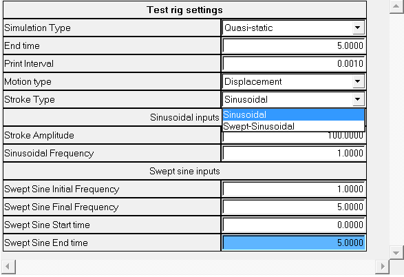
Figure 5.It is important to note here that a Transient analysis is needed if you wish to plot damper velocity characteristics.Note: In the component test rig, you can simulate the impact of road excitations on the suspension by selecting one of the options in the Motion type drop-down in the Analysis Wizard. The motion is applied to the axle in the test rig. Currently, the following two options are supported:- Sinusoidal Input
- Sinusoidal input allows the user to apply a time-invariant
frequency based displacement/velocity to understand the response
of the suspension. The response is governed by the following
equation,
Y=A sin(ωt)
Where, A is the amplitude of the stroke, ω is the constant angular frequency and t is the current time.
- Swept-Sinusoidal Input
- Swept sinusoidal input allows the user to apply a time-variant
frequency to the axle. The swept sinusoidal response is governed
by the following equation,
Y=A sin(thetha(t))
where A is the amplitude, and thetha(t) =
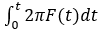
Based on the values, input for the start and end time for swept sine analysis by the user, F(t) is considered to vary according to the following equations.
F(t)=0 0<t< tstart
F(t)=ωinit + (ωfinal - ωinit)(t-tstart) tstart < t < tend
F(t) = ωfinal t > tend
For the time starting from tstart to tend, the frequency is assumed to vary linearly from ωinit to ωfinal.
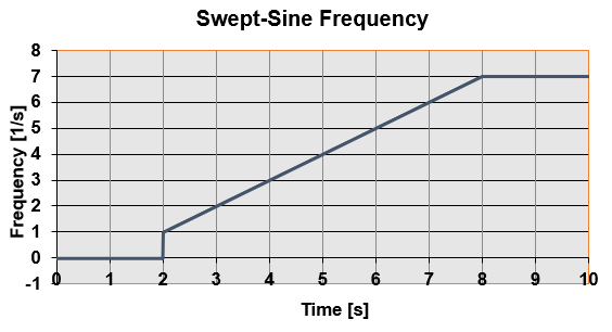
Figure 6.The above graph shows an example of a frequency input where the frequency varies linearly from 1Hz at t=2sec to 7Hz at t=8sec.