Stress
gradient effect based on FKM guideline method.
It is supported for both shells and solid elements. For solid elements, the stress
gradient effect is only available with grid point stress in fatigue analysis using
results of static analysis. For solid elements, SURFSTS field on
FATPARM is automatically set to GP when
Stress Gradient effect is activated.
The Stress Gradient method is supported for Uniaxial and Multiaxial SN, EN and FOS
Fatigue. It is not supported for Weld, Vibration, and Transient Fatigue
analyses.
FKM Guideline Method
In the FKM guideline method, stress gradient effect is considered by increasing
fatigue strength by a factor calculated using a rule in FKM guidelines. In HyperLife implementation of FKM guideline method, 6 components of a
stress tensor at each time step is reduced by the factor provided by FKM
guidelines.
To activate Stress Gradient effect using FKM guideline method, the
GRD field on FATPARM should be set to
GRDFKM.
The following steps are followed to reduce stresses at the surface to take stress
gradient effect into consideration.
Calculate stress gradient of 6 components of a stress tensor,
, at each time step after
linear combination of stress history. z-direction is an outward surface
normal. For a solid element, the gradient is calculated by finite difference
between stress at surface and stress at 1mm below the surface. The stress at
1mm below surface is an interpolated stress from grid point stresses of an
element of interest. In case of 2nd order solid elements, only
grid point stresses at corners are used for interpolation. For shell
elements, the gradient is calculated from stresses of both layers and its
thickness.
Using the stress gradient obtained in Step 1, a gradient of equivalent
stress in the surface normal direction,
, is calculated in an
analytical way at each time step. The equivalent stress can be either von
Mises stress or absolute maximum principal stress.
The related stress gradient, is calculated using the following
normalization.(1)
Apply the correction factor to the surface stress tensor to obtain
reduced surface stress. Apply the same to corresponding strain tensor to obtain
reduced strain tensor when EN fatigue analysis is to be carried out with
nonlinear analysis.(2)
Correction Factor Calculation
Correction factor calculation is based on relationship between and described in the FKM guidelines.
According to FKM guidelines, the stress correction factor is determined by:
Table 1. Example values for Constants and
Constants
Stainless Steel
Other steels
GS
GGG
GT
GG
Wrought Al-Alloys
Cast Al- Alloys
0.40
0.50
0.25
0.05
-0.05
-0.05
0.05
-0.05
2400
2700
2000
3200
3200
3200
850
3200
Where,
GS
Cast Steel and Heat Treatable cast steel for general purposes.
GGG
Nodular Cast Iron.
GT
Malleable Cast Iron.
GG
Cast Iron with lamellar graphite (grey cast iron).
is UTS in MPa and dimension of is mm. HyperLife takes care of the
unit system for and through stress units defined in
MATFAT and stress unit and length unit defined in
FATPARM. and values are user input in MATFAT
after keyword STSGRD. Since the stress gradient has to be
calculated in length dimension of mm, define the length units so that HyperLife can properly locate a point that is 1mm below the surface. If is negative, is set to 1.0. If is greater than 100 mm-1, is set to 1.0 with a warning message.
User-defined Relationship
User-defined relationship between and can be specified through TABLES1
Bulk Data. Pairs of (xi,yi) = ( , ) can be defined on the TABLES1
entry. A TABLES1 that defines the relationship between and should be referenced in MATFAT
after keyword STSGRD. If falls outside the range of xi, extrapolation
behavior follows usual TABLES1 behavior. This means that can be lower than 1.0 when is negative depending on how is treated when being negative or greater than
100mm-1. The user-defined relationship takes precedence over the one in FKM
guidelines.
Critical Distance Method
To activate Stress Gradient effect using Critical Distance method, the
GRD field on FATPARM should be set to
GRDCD.
Small stress concentration features or geometries with high stress gradients are less
effective in fatigue than larger features or smaller gradients with the same maximum
stress. A plate with a small hole, say 0.1mm, will have a much longer fatigue life
than one with a large hole of 10mm even though both plates have the same stress
concentration factor and maximum stress. In conventional fatigue analysis, the
stress gradient effect is taken into account by using an empirical fatigue notch
factor, Kf, rather than the stress concentration factor
Kt. Since there is no concept of a Kt or
nominal stress in a finite element model stress gradient effects are considered
directly. All of the holes have the same maximum stress, three times the nominal
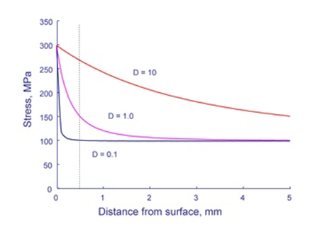
stress. Figure 1. Stress distribution in a plate for three different hole sizes
Figure 1 that the stresses are independent
of size only at the edge of the hole and vary far from the hole. The dashed line in
the figure is drawn at 0.5mm. Here the stresses increase as the size of the hole
increases. Suppose crack nucleation mechanisms result in a crack with a size of
0.5mm. For the smallest hole, 0.1mm, the stress available for continued growth is
only 100 MPa, the nominal stress. The same size crack is subjected to a stress of
275 MPa in the larger hole, nearly equal to the maximum stress.
For nucleation of a crack around a hole of different sizes, it is useful to think
about a process zone for crack nucleation. Materials are not continuous and
homogeneous on the size scale that crack nucleation mechanisms operate. The grain
size of the material is a convenient way to visualize the fatigue process zone.
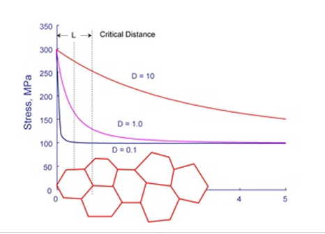
Figure 2 shows the grain size superimposed
on the stress distribution from Figure 1. What is the stress in the process
zone? A simple first approximation would be to take the stress in the center of the
grain. Thus, a stress of 275 MPa would be used to compute the fatigue life of a 10mm
hole and a stress of 100 MPa would be used for the 0.1mm hole. Figure 2.
The modern view of fatigue is that when a material is stressed at the fatigue limit a
microcrack will form but not grow outside of the process zone. Stress gradient
effects are included in the fatigue analysis in a very simple and straightforward
manner. In Critical Distance method, stresses and strains at a distance L/2 (Point
Method) from the surface are used rather than the surface stresses and strains. For
solid elements, the stress and strain at L/2 below surface is an interpolated stress
and strain from grid point stresses and strains of an element of interest. In case
of 2nd order solid elements, only grid point stresses and strains at corners are
used for interpolation.
The critical distance can be expressed in terms of the threshold stress intensity, , and fatigue limit range, , as:(3)
The critical distance is a unique material property. If the critical distance of the
material in use is known, user can input the critical distance in
MATFAT after keyword STSGRD. When you
input the critical distance, it is important to define dimension of length in
MATFAT as well. Computing the critical distance from the
threshold stress intensity, however, is difficult because the threshold stress
intensity, particularly for small microcracks, is usually unknown. Fortunately,
there is a good direct correlation between the critical distance and
fatigue.(4)
If you do not directly input the critical distance, HyperLife uses
Equation 4 to estimate the critical distance
in SN fatigue analysis. Fatigue limit is taken after the SN curve adjustment. Dimension of
L is mm.
In EN fatigue analysis, the fatigue limit is approximated in the following
manner.(5)
(6)
Where,
Fatigue strength coefficient.
Reversal limit of endurance.
Young’s modulus.
If is 0 or the calculated is greater than 0.2mm, will be set to 0.2mm. In case of shell elements, the
maximum calculated is thickness/4.
Input to Activate Stress Gradient Effect
Choose a method (FKM guideline or Critical Distance) to use on the
GRD field after keyword STRESS in
FATPARM. If FKM guideline method is chosen, the equivalent
stress method to calculate stress
gradient should be specified on the SCBFKM field in
FATPARM. Material properties required for stress gradient
effect are to be input after keyword STSGRD in
MATFAT.