Manage Scopes in the Project Browser
Use the options in Project Browser context menu to manage scopes after running a simulation.
-
From the Project Browser, right-click the scope block name and select from the
following options on the context menu:
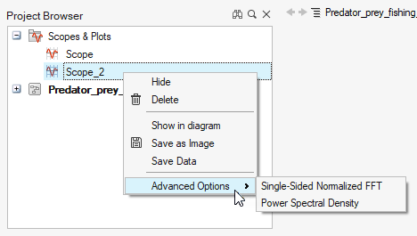
Option Description Hide Shows the plot that has been created. Delete Deletes the plot window, not the Scope block. Show in Diagram Highlights the selected block in the diagram. 
Save as Image Saves the plot as an image .png or .bmp file. Save Data Saves the data that is displayed in the plot as a .csv or .mat file. This option works for plots with and without subplots. Displays data in a frequency domain for the Scope block. Select the Single-Sided Normalized FFT or Power Spectral Density option, then enter a sampling frequency in the Input Dialog.
A new window is generated with a frequency-domain plot and is named based on the primary scope window followed by FFT or PSD.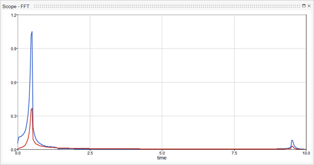
Assumptions for the Frequency-Domain Calculation
The initial time for the computation of the FFT and the PSD is internally set to zero:t=t-min (t)
The algorithm conducts data resampling according to the sampling period, which is the inverse of the sampling frequency:
The method to transform data from a time to frequency domain deletes time duplicates because the Activate simulator may generate two or more successive data points with the same time instant.
Some phenomena cannot be taken into account, such as aliasing and leaking, since this feature provides an introductory functionality to seamlessly visualize the data in frequency domain. For further customization of parameters in the frequency domain, OML functions for signal processing are available to be used through scripting.
Computation of FFT
If the number of samples is even, the formulation is as follows:
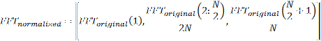 Where N is the number of samples of the signal. The correspondent frequency vector is:
 If it is odd:
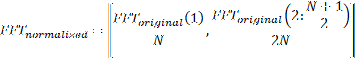 Where N is the number of samples of the signal. The correspondent frequency vector is:
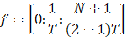
Computation of PSD
If the number of samples is even, the FFT and the frequency vector are calculated like it was described above, while the PSD is:
Where N is the number of samples of the signal.
If it is odd, the FFT and the frequency vector are calculated like it was described above, while the PSD follows the same formula as if the number of samples was even.
Where N is the number of samples of the signal.