
Place the following eMotors blocks in your diagram:
•PWM Brushless Servo Amplifier
Flip the Rotary Absolute Encoder and Hall Sensor blocks using the Edit > Flip Horizontal command. Then arrange the blocks and wire them together, as shown below.
In this application, there is no reason to reset the integration of the PID Controller-Digital, so a 0 const is wired to Integrator Reset (High) to disable it. In other applications, repetitive control may be used, and Integrator Reset (High) may be required to re-initialize the control between repetitions.
A value of 100 amps is chosen for this example to make certain saturation does not occur. Later on, you might possibly measure currents encountered in this simulation under highest load conditions and set a more appropriate current limit for the final design.
Next, place the following eMotor blocks in the diagram:
Flip the Rotary Encoder and Rotational Load blocks and arrange the blocks as shown below:

Connect the Rotor Displacement output on the Brushless DC Motor-Digital these three blocks: the shaft angle input on the Hall Sensor block, the displacement input of the Rotary Absolute Encoder, and the Rotor Displacement input on the Rotational Load.
Connect the outputs of the PWM Brushless Servo Amplifier to the corresponding inputs of the Brushless DC Motor-Digital. Connect the Load Reaction Torque output on the Rotational Load to the Load Reaction Vector input on the Brushless DC Motor-Digital.
Lastly connect a const block with 0 set value to the load disturbance input on the Rotational Load. If there were other torques related to influences that could not be directly represented by the set parameters of the rotary load model, the load disturbance input provides a method for introducing such torques. For the target tracker, it might be conceivable to introduce torque noise induced by structural vibrations of the tracker mount. If the mount were part of a satellite payload, such vibrations could arise from solar array positioning systems. Noise profiles with specific power spectral densities can be generated in Embed using the Random Generator blocks and transferFunction block. Coefficients of the transfer function are determined by applying spectral factorization techniques to the known PSD.
Next, insert a Park Transform and a Clark Transform into the diagram and connect them as shown below:

Encapsulate the blocks in Current Sense. Then label the input and output connector tabs as shown below:

Flip the block and connect the ias and ibs outputs on the Brushless DC (BLDC/PMSM) Motor to the corresponding a and b inputs on the Current Sense. Connect the displacement output of the Rotary Encoder to the angle input of the Current Sense.
Connect the Load Displacement output on the Rotational Load to the displacement input of the other Rotary Absolute Encoder.
Complete the wiring by connecting the output on Current Sense to the current sense input on the PWM Brushless Servo Amplifier and the rate output on the Rotary Absolute Encoder to the tach input on the PWM Brushless Servo Amplifier, as shown below:

This diagram represents a cascade control loop. The inner loop senses and controls current; the middle loop senses and controls velocity; and the outermost loop senses and controls position.
Now the entire diagram must be collapsed into a single compound block named X Axis Servo. Reduce the number of inputs and outputs on X Axis Servo to one, and label the input connector commanded LOS and output connector actual LOS.
Then drill into X Axis Servo and make certain that the commanded LOS is connected to the command input on the PID compensator block and the displacement output of the Rotational Load is connected to the actual LOS output of the compound block.
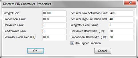
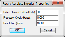
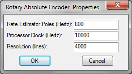
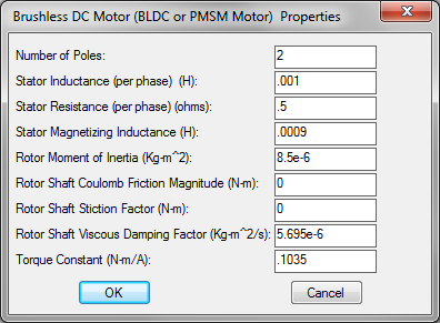
While still in the X Axis Servo, open the dialog boxes of each block and enter the following parameter values as specified by the design input.
PID Controller (Digital) block
PWM Brushless Servo Amplifier block

Rotary Encoder block that feeds back to PID Controller (Digital) block
Rotary Encoder block that feeds back into the PWM Brushless Servo Amplifier block
Brushless DC (BLDC/PMSM) Motor block
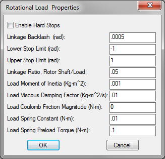
Rotational Load block
This completes the x-axis of the servo controller. Completing the y-axis takes only a couple of keystrokes, as all dynamics for this axis mirror the x-axis. Make a copy of X Axis Servo using the Edit > Copy command. In the dialog box for the newly-created X Axis Servo, change the block name to Y Axis Servo. At this point, there are two servo controllers in your diagram: an x-axis and a y-axis servo controller.
Next, create the pipeline image processor. For this processor, the dominant feature is the sample frame rate of 60 Hz. Place two sampleHold blocks and a pulseTrain block in your diagram, as shown below:

In the pulseTrain block, set the time between pulses to 1/60 (0.0167). Then encapsulate the three blocks in a compound block and name it Focal Plane Pipeline Processor.

Create the following block configuration:

This creates an elliptical motion for the target in the X-Y plane. Frequency for each axis is the same (1 rad/sec); however, phase differs.
Collapse the blocks into a compound block and name it Target:

Connect the compound blocks as shown below:

The command line of sight (LOS) is set to the target angle that is determined by the pipeline processor. The difference between the target angle and actual line of sight is calculated using summingJunction blocks that provide focal plane error. The error is converted into degrees using unitConversion blocks.