Magnet (unidirectional): demagnetization curve (Hc, Br)

Presentation

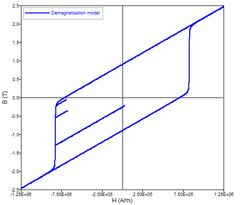
This model ( Nonlinear magnet described by H_c and the B_r module ) defines a nonlinear B(H) dependence with taking into account of demagnetization, wherever the curve knee is.

Main characteristics:

• the mathematical model and the direction of magnetization are dissociated
• a single material for description of several regions

Mathematical model

In the direction of magnetization the model is a combination of a straight line and an arc tangent curve.

The corresponding mathematical formula is written:

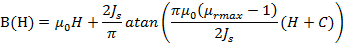
with: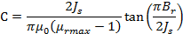

where:

• μ₀ is the permeability of vacuum, μ₀ = 4 π 10^-7 (H/m)
• μ_rmax is the maximal relative permeability of material
• B_r is the remanent flux density (T)
• J_s is the saturation magnetization (T)

The shape of the B(H) dependence in the direction of magnetization is given in the opposite figure.

In transversal directions one can write:

B_⊥(H)= μ₀μ_r⊥H_⊥

where μ_r⊥ is the transverse relative permeability

Direction of magnetization

The various possibilities provided to the user are the same ones as those presented in § Magnet (unidirectional): linear approximation.

Demagnetization during solving

With this non-linear model, it is now possible to taking in account demagnetization during solving by checking the thick that is provided for. This model is based on a static Preisach model, and can be applied in all over the B(H) law of the magnet:

To use this new model with a solved project :

Example of results

Here is a surface permanent magnets motor 3D

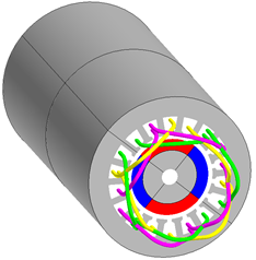
Figure 1. Full device

For a control angle $\Psi =\left[ 0 ; \frac{\pi }{6} ; \frac{\pi }{4} ; \frac{\pi }{3} \right]$ , we can see that there is a local effect on the remanent flux density, but the repartition depends of the angle $\Psi$ .

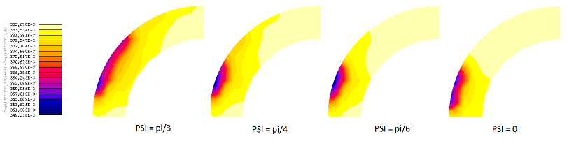
Figure 2. Br in the magnet

This local effect can bring some effect on global values like torque or EMF.

Figure 3. E.M.F with and without demagnetization for $\Psi =\frac{\pi }{4}$