Computation of inductance matrices
Introduction
Since version 2020, Flux is able to compute the time evolution of the self and mutual inductances (apparent and incremental) of every device containing stranded conductor circuit components. This computation, which previously obliged the user to develop a Python script, has now been automatized.
This new feature, which is now available for Transient Magnetic applications, consists of a series of Magnetostatic simulations that are automatically batch-processed by Flux, requiring no additional intervention from the user. In this way, the set of self and mutual inductances of the device is obtained from the evaluation of the magnetic flux linked to the coils performed during these simulations.
Once the inductances are computed, the yielded values are stored as exportable Flux Input/Output Parameters. The user may easily employ them to display their time evolution or to assemble a time-varying inductance matrix.
A typical application for this new tool is the control of rotating electric machinery. For instance, the inductance matrices computed by Flux could be used to represent a machine in a system simulation software such as Altair Activate®.
How to use it
This feature is available in the 2D module of Flux for solved Transient Magnetic projects, while in post-processing mode. Under such conditions, to launch an inductance computation in Flux:
- In the Computation menu, choose command Computation of Inductance Matrix;
- Select the inductance type to be evaluated: apparent, incremental
or apparent and incremental;The definitions of apparent and incremental inductances Lapp and Lincr are shown in Figure 1.
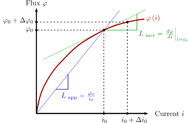
Figure 1. Apparent and incremental inductances Lapp and Lincr of an electromagnetic device, obtained from its characteristic function φ(i) at an operating point (φ0, i0). - Select the source coils (i.e., the stranded conductor coils generating a flux);
- Select the target coils (i.e., the stranded conductor coils
subjected to a flux);Note: For instance, if a project has two coils, the inductance matrix contains four terms: L11, M12, M21, and L22. If the user selects the 1st as a source coil and both the 1st and 2nd as target coils, Flux will evaluate the following two terms : L11, M12.
- Provide a string of characters (for example, PREFIX), which will take part in the names of the Input/Output Parameters to be created by Flux to store the results;
- Click OK to run the computation;Note: The serie of Magnetostatic simulations is distributed over a certain number of Flux instances, which is automatically determined accordingly with the number of cores set in the Options in the Supervisor. To configure the number of cores used, go to Supervisor > Options > System Options > Parallel computing.
- By the end of the computation, the results can be found in the list of Input/Output Parameters
with names PREFIX_APP_X_Y (for apparent inductance computations) or
PREFIX_INCR_X_Y (for incremental inductances computations).Note: The user may then continue by drawing 2D curves from the Input/Output Parameters to observe the time evolution of the results. He may also export them to a file, making them available to other software.
An application example
An inductance computation using this new feature has been performed in the case of the device shown in Figure 2, which is available in the catalog of examples of Flux Supervisor (under Technical tutorials, Brushless IPM motor). The device is a three-phase, eight-pole synchronous machine with a permanent magnet rotor.
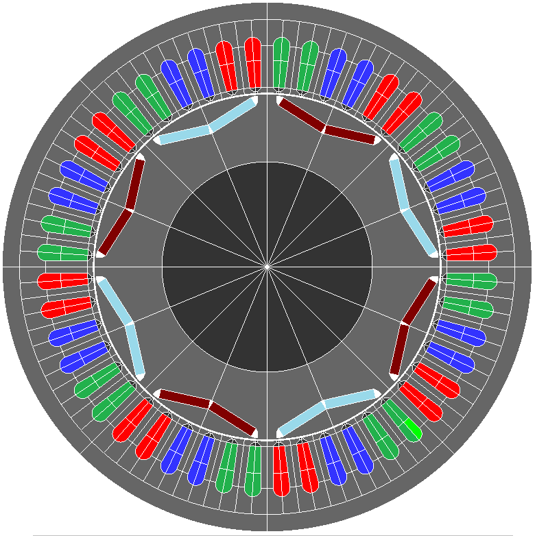
Figure 2. A three-phase, eight-pole synchronous machine with a permanent magnet rotor.
In this example, the apparent inductance matrix has been computed with Flux in the case of an imposed rotor speed of 1200 rpm. Each stator coil a, b, and c was simultaneously designated as a source and as a target coil. These windings are fed by current sources Ia, Ib et Ic in accordance with the circuit shown in Figure 3:
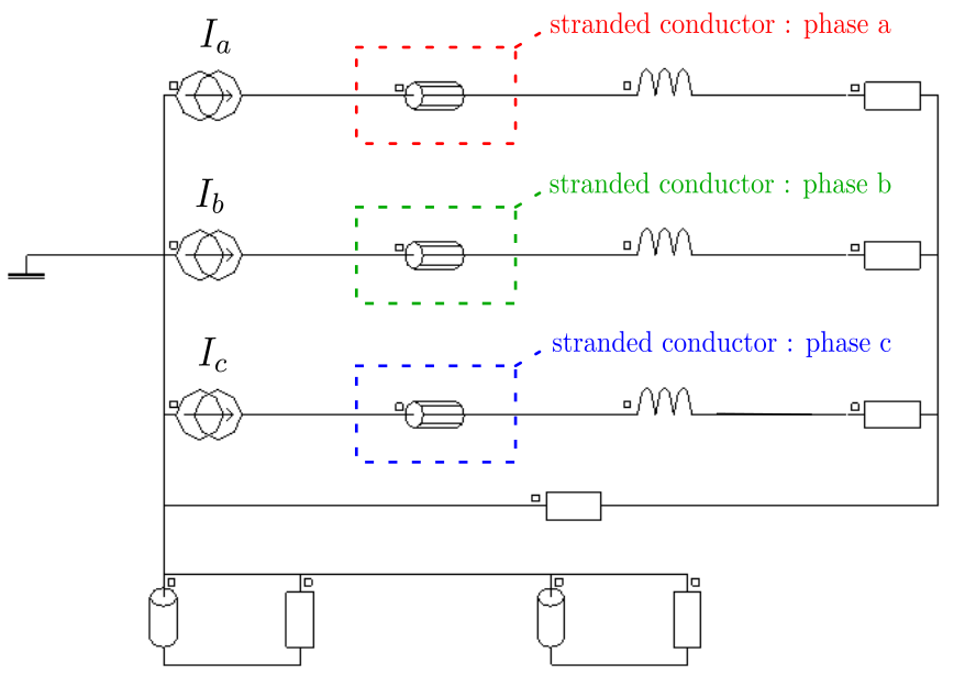
Figure 3. The electric circuit in Flux modeling the synchronous machine shown in Figure 2. Notice the three Stranded Coil Conductor circuit components that model the stator windings of the machine.
The time variations of apparent self inductances La, Lb and Lc and of apparent mutual inductances Mab=Mba, Mbc=Mcb and Mac=Mca were computed by Flux. The results are shown in Figure 4.
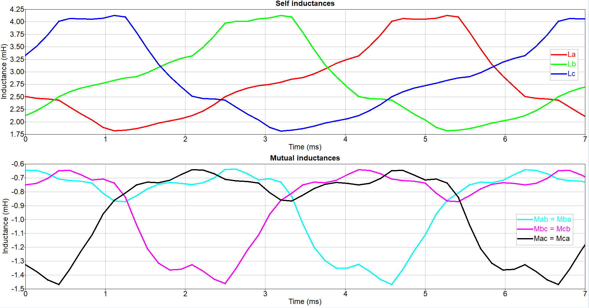
Figure 4. Time evolution of the self and mutual inductances of the synchronous machine shown in Figure 2 computed by Flux. The results stored in the Input/Output Parameters were exported and treated with Altair Compose® to generate this picture.
At each time step, the magnetic flux components φa, φb and φc linked to the three stator coils are related to the apparent inductances by the following equation:
In this last equation, terms φ0a, φ0b and φ0c represent the magnetic flux components produced by the magnets of the machine and concatenating the stator windings.
Limitations
As already mentioned, this feature is only available in the 2D module of Flux for Transient Magnetic applications. A few additional constraints must also be satisfied by Flux projects:
- Anisotropic materials and non-linear magnets are not allowed;
- Hysteretical materials are not allowed;
- Line regions are not allowed;
- Scenarios containing geometric parameters are not allowed;
- Circuit-dependant formulae are not allowed.
References
Transient Magnetic application: principles