Study domain limits, generalities
Electro magnetic phenomena
In the study of electromagnetic phenomena it is necessary to model both the device and the surrounding air. In fact, the quantities studied in electromagnetics (electric fields, magnetic fields), are not considered null in air or in a vacuum, contrary to other physics disciplines, mechanics, for example, where air is not taken into account.
Finite element method
The finite element method is based on the subdivision of the entire study domain in a finite number of sub domains of finite size.
The physical problem is governed by a differential equation or with partial derivatives that should be satisfied on all the points of a domain. To ensure the uniqueness of the solution, boundary conditions on the outer edges must be imposed.
Thus, to solve a problem with the finite element method, it is necessary to:
- set limits on the device model, i.e. to define the limits or boundaries of the domain,
- impose boundary conditions on the edges, i.e., to define the values of the state variable (potential, temperature) on the boundaries of the domain.
Apparent contradiction
The finite element method requires limits on the problem region, while the electromagnetic phenomena are unlimited.
In other words, open domains cannot be modeled by the finite element method, because it is impossible to subdivide an infinite domain into a finite number of finite sub-domains.
Study domain limits: different methods
To offset this contradiction, different methods can be used.
The first method (the truncation method) consists of closing the study domain with an outer boundary sufficiently far away from the device so as not to interfere with the results.
The second method consists of using a transformation that converts the open domain into a closed domain.
These two methods are described in the following paragraphs.
Study domain limits: truncation method
The truncation method consists of closing the study domain with an outer boundary sufficiently far away from the device so as not to interfere with the results.
The device is placed inside an air–filled box, and infinity is approximated by a closed and remote truncation boundary. The size of the air-filled box is adjusted so that the effects of the truncation boundary approximation can be neglected.
The user must determine the quantity of air to model around the device, i.e., he or she must evaluate the distance at which the computed fields become negligible.
Truncation method: disadvantages
The truncation method has certain disadvantages:
- relatively high cost in terms of numbers of unknowns
- negligible field values near the truncation boundary
Modeling infinity: using a transformation
To compensate for these disadvantages, a second method consists of using a transformation that converts the open domain into a closed domain.
The basic idea is to transform the open domain into a closed domain because the open domain cannot be meshed.
Use of a transformation, principle
The intial space is decomposed into two domains:
- a closed interior domain, Eint
- an open exterior domain, Eext
The initial space, with open borders, is transformed into a final space with closed borders, in the following way:
- the interior domain (Eint) is not modified
- the exterior domain (Eext) is linked to a closed domain (Eext_image) through a spatial transformation T.
Thus, the final space is composed of two domains:
- a closed interior domain Eint
- a closed exterior domain Eext_image
These two (closed) domains are meshed with classical finite elements.
Illustration

Use of a transformation, principle (continued)
To take into account the transformations in the equations, we suppose that :
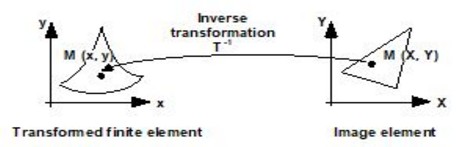
- the finite elements formulations are not modified (the state variable of the initial domain and the state variable of the image domain are equal)
- new types of finite elements (transformed finite elements) are able to model infinity.
Illustration: Representation of the exterior domain

Choice of the transformation
Theoretically several space transformations can be used. The transformation of the real space into an image space must be bijective. It must also have properties of continuity and derivability on and between the elements, etc.
In practice, the transformations used in the software take into account various efficiency criteria: quality of the solution obtained for a number of elements or unknown factors, simplicity of implementation and so on.