Adaptive solver: about
Introduction
The finite element method of analysis offers a numerical solution for physical phenomena described by partial differential equations. For this, it relies on a sampling of the studied domain that is called mesh. The denser the mesh of the studied domain, the more accurate the numerical solution will be, but this is at a high cost in terms of computer memory requirements.
It is therefore essential to generate a mesh that should be refined in the zones that require it and loose in the rest of the domain. In other words, the mesh must be adapted, both, to the geometry and to the physics demands of the problem.
History
Over the last years, considerable effort has been made in order that the Flux software could automatically generate a qualitative mesh.
The first stage was to set up the aided mesh, which permits the user to obtain a mesh adapted to the geometry of the problem.
Today, the Flux software offers the adaptive solver. This process facilitates automatically refined mesh in the locations where the physics of the problem require it.
Description
The adaptive solver is a process that permits modeling a problem by means of an adaptive mesh. This mesh presents sizes of elements, which correspond to the local behavior of the considered physics.
In the zones requiring a finer analysis of the studied phenomenon, this translates by:
- A tightening of the meshes
- A diminution of the finite elements size
| No-adapted mesh | Adapted mesh |
|---|---|
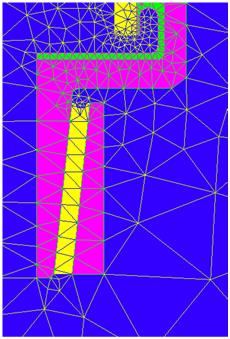
|
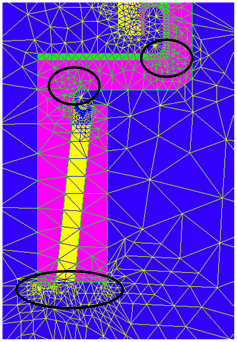
|
Limitations / Restrictions in 2D
Here are some restrictions:
- The adaptive solver is reserved to the applications:
- Magneto Static 2D
- Electro Static 2D
- Steady State AC Magnetic 2D
- The adaptive solver does not work with the:
- mechanical sets of the « compressible » type
- anisotropic, non linear regions
- It is not advisable to use the mapped mesh with the adaptive solver
- As for all solvers, one should start from an initial mesh
Limitations / Restrictions in 3D
Since Flux 12.1, adaptive solver is available for the 3D applications:
- Electro Static 3D
- Magneto Static 3D
In 3D, the limitations of the adaptive solver are:
- mechanical sets
- mapped mesh or extrusion mesh
- physics with surface of type “Air Gap region”
Note that 2nd order mesh will automatically be created in order to compute relevant local errors.