ACU-T: 2400 Supersonic Flow in a Converging-Diverging Nozzle
Prerequisites
This tutorial provides instructions for modeling a supersonic flow in a converging diverging nozzle using HyperWorks CFD. Prior to starting this tutorial, you should have already run through the introductory tutorial, ACU-T: 1000 Basic Flow Set Up, and have a basic understanding of HyperWorks CFD and AcuSolve. To run this simulation, you will need access to a licensed version of HyperWorks CFD and AcuSolve.
Prior to running through this tutorial, click here to download the tutorial models. Extract ACU-T2400_CD_Nozzle.hm from HyperWorksCFD_tutorial_inputs.zip.
Problem Description
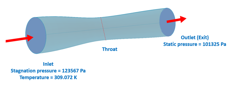
Figure 1.
The exit to throat area ratio of the nozzle is 1.5. The radius at the inlet is 0.892 m, while the radius at the outlet is 0.691 m. The inlet stagnation pressure and the inlet temperature are 123,567 Pa and 309.072 K, respectively. The static pressure at the outlet is set to 101,325 Pa. The fluid in this problem is air, where the flow is assumed inviscid (viscosity and conductivity are zero) and density is based on the ideal gas model.
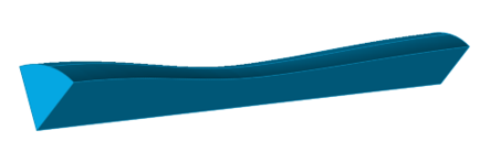
Figure 2.
The AcuSolve simulation will be set up to model a transient supersonic flow where the flow variables reach an asymptotic state to determine the stable flow solution.
Start HyperWorks CFD and Open the HyperMesh Database
-
From the Home tools, Files tool group, click the Open Model tool.

Figure 3.The Open File dialog opens.
Validate the Geometry
The Validate tool scans through the entire model, performs checks on the surfaces and solids, and flags any defects in the geometry, such as free edges, closed shells, intersections, duplicates, and slivers.
Figure 4.
Set Up Flow
Define Material Properties
-
From the Flow ribbon, click the Material Library tool.

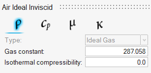
Figure 5.The Material Library dialog opens. -
Click
 to add a new ideal gas model.
-
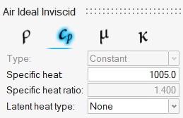
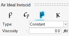
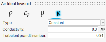
Rename the model to Air Ideal Inviscid.
Figure 6.
Set Up the Simulation Parameters and Solver Settings
-
From the Flow ribbon, click the Physics tool.

Figure 7.The Setup dialog opens. -
Under the Physics models setting:
- Select the Supersonic radio button under Single phase flow.
- Set the Ideal gas model to Air Ideal Inviscid.
- Set the Time step size to 0.000125.
- Set the Final time to 0.3125.
- Verify that the Turbulence model is set to Laminar.
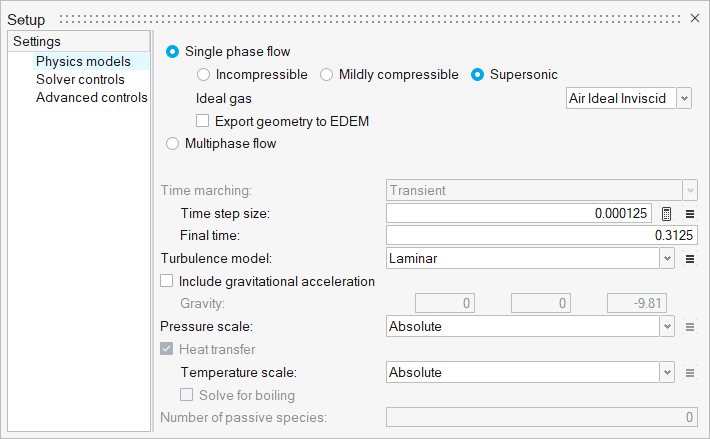
Figure 8. -
Set the Maximum stagger iterations to 5.
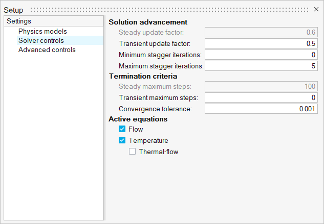
Figure 9.
Verify the Material Selection
-
From the Flow ribbon, click the Material tool.

Figure 10. -
Click
 on the guide bar.
Define Flow Boundary Conditions
-
From the Flow ribbon, Pressure
tool group, click the Stagnation Pressure tool.

Figure 11. -
Click on the inlet face highlighted in the figure below.
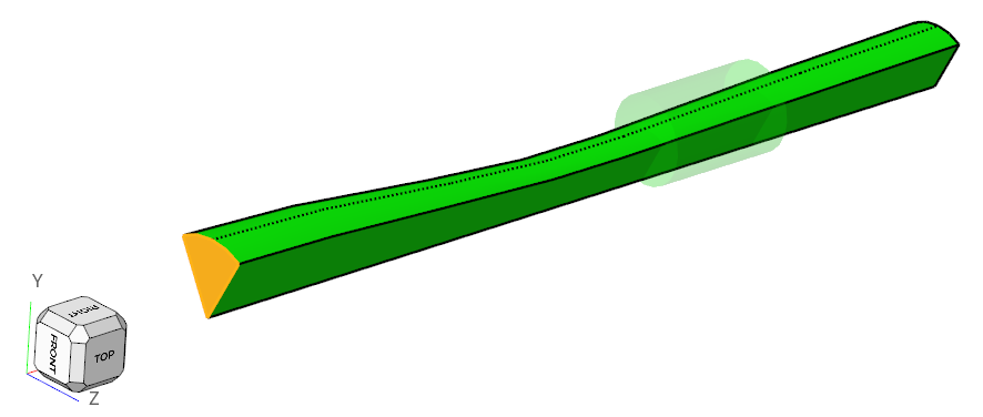
Figure 12. -
In the microdialog, enter the following values for the
stagnation pressure and temperature.
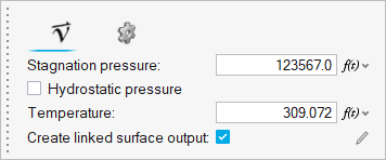
Figure 13. -
On the guide bar, click
 to execute
the command and exit the tool.
to execute
the command and exit the tool.
-
Click the Outlet tool.

Figure 14. -
Select the face highlighted in the figure below, enter the
101325 as the static pressure value, and then click
on the guide bar.
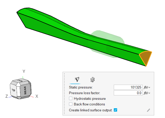
Figure 15. -
Click the Slip tool.

Figure 16. -
Select the face highlighted in the figure below and then click on the
guide bar.
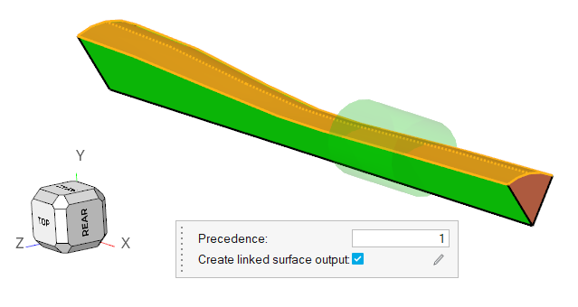
Figure 17. -
Click the tool.

Figure 18. -
Select the face highlighted below as the Source.
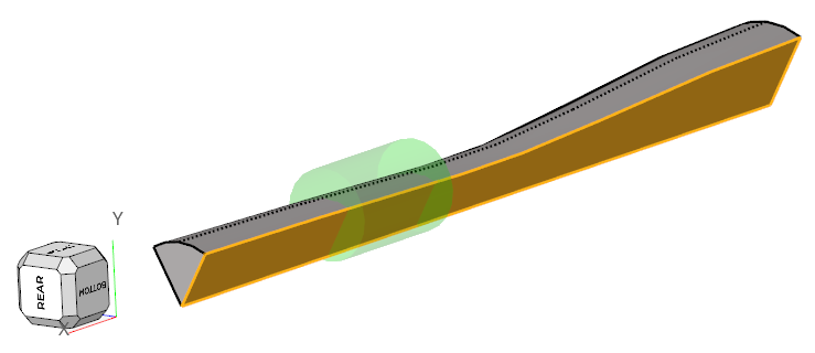
Figure 19. -
Click Target on the guide bar
then select the opposite face.
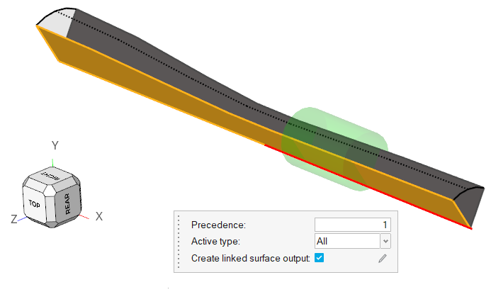
Figure 20. -
Click on the guide bar.
Generate the Mesh
-
From the Mesh ribbon, click the
Volume tool.

Figure 21.The Meshing Operations dialog opens.Note: If the model has not been validated, you are prompted to create the simulation model before running the batch mesh. -
Accept all other default parameters.
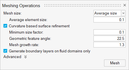
Figure 22.
Run AcuSolve
-
From the Solution ribbon, click the Run tool.

Figure 23. -
Leave the remaining options as default and click
Run to launch AcuSolve.
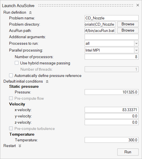
Figure 24.The Run Status dialog opens. Once the run is complete, the status is updated and you can close the dialog.Tip: While AcuSolve is running, right-click on the AcuSolve job in the Run Status dialog and select View Log File to monitor the solution process.
Post-Process the Results with HW-CFD Post
In this step, you will check the contours of pressure on a mid slice plane.
-
Select the AcuSolve log file in your problem
directory to load the results for post-processing.
The solid and all the surfaces are loaded in the Post Browser.
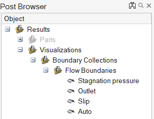
Figure 25. -
Move the animation slider to the end to load the last time step data.

Figure 26. -
Click the Slice Planes tool.

Figure 27. -
In the slice plane microdialog, click
 to
create the slice plane.
to
create the slice plane.
-
Click
 and set the Legend location to Upper
Center, the Legend Orientation to
Horizontal, and the Colormap name to
Rainbow Uniform.
and set the Legend location to Upper
Center, the Legend Orientation to
Horizontal, and the Colormap name to
Rainbow Uniform.
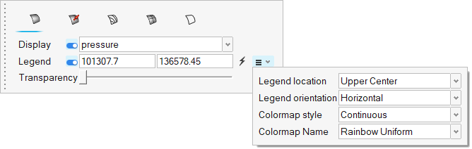
Figure 28. -
Click on the guide bar.
-
In the Post Browser, hide the Flow
Boundaries surfaces to display the pressure contours on the
slice plane.
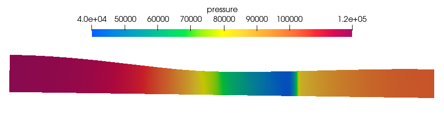
Figure 29.Similarly, you can display the Mach number contour.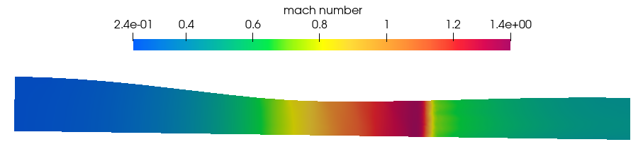
Figure 30.