Post-Processing

Post-process the simulation results by creating visualizations and measurements.

When you navigate to the Post ribbon, the model used for the pre-processing setup is cleared. To load a model for post-processing, open a log file from a completed AcuSolve run.
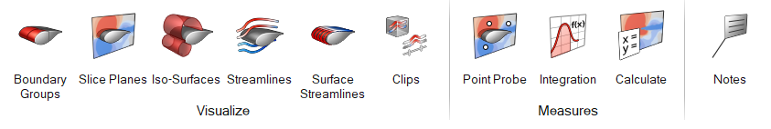
Attention: The icons shown on the ribbon below are used to complete this workflow. Click an icon to learn more about the tool.
Use the Boundary Groups tool to create a group of surfaces and define display properties. These surface groups can be utilized to group boundaries as required and define specific display properties. Use the Streamlines tools to create derived geometry streamlines which represent particle paths in a flow field. You have to define participating solids, seed points, and vectors from which streamlines are computed as well as the integration direction. There are various methods to generate seed points. Use the Slice Planes tool to create derived geometry by slicing solids on a plane and defining display properties. The result of slicing is a 2D planar face. Use the Iso-Surfaces tool to a create a derived geometry surface with a specific constant scalar value and define display properties. The shape of the iso-surface is dependent on domains and flow field. Use the Surface Streamlines tool to create streamlines on surfaces with given seeds. Use the Probe Points tool to define a point or set of points at specific co-ordinates and probe/query results. This is useful for verifying experimental results with simulation result. Use the Calculate tool to create new field quantities using a python expression. The new fields can be derived from existing fields or be completely independent of other results in the dataset. Use the Integration tool to get integrated quantities on surfaces, solids, volumes, slice planes, and iso-surfaces. Use the Box and Scalar Clip tools to hide portions of your model, allowing you to better view areas of interest. Use the Notes tool to add annotations in the modeling window.