ACU-T: 6105 Single Particle Sedimentation – Effect of Lift and Torque
Prerequisites
This tutorial demonstrates the effect of lift and torque forces on a non-spherical particle falling through a fluid using AcuSolve-EDEM bidirectional coupling. Prior to starting this tutorial, you should have already run through the introductory HyperWorks tutorial, ACU-T: 1000 Basic Flow Set Up and ACU-T: 6100 Particle Separation in a Windshifter using Altair EDEM, and have a basic understanding of HyperWorks CFD, AcuSolve, and EDEM. To run this simulation, you will need access to a licensed version of HyperWorks CFD, AcuSolve, and EDEM.
Prior to running through this tutorial, click here to download the tutorial models. Extract the files from the folder named ACU6105_EDEM_Sedimentation located in HyperWorksCFD_tutorial_inputs.zip.
Problem Description
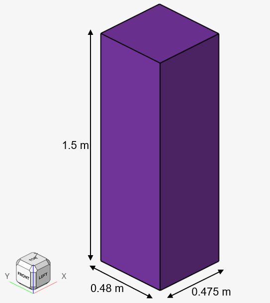
Figure 1.
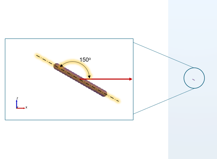
Figure 2.
AcuSolve-EDEM bidirectional coupling is used to model the interaction between the fluid and particle. In this tutorial, the Rong drag model in conjunction with the Ganser non-spherical drag-coefficient model is used such that the effect of non-spherical shape is considered. The length scale used for factoring in the shape of the particles is the aspect ratio. A cylindrical particle with an aspect ratio of 9.242 (L/D = 0.05 m/0.00541 m) is used for this simulation.
This tutorial also introduces you to the concept of generating particles in EDEM at a specific location and with a specific orientation. When defining the particle factory, you have the option to define certain properties of particles such as velocity, angular velocity, position, orientation, temperature, and so on. Properties such as orientation and position can be defined by you or set to random. The steps listed below illustrate the general process for calculating the orientation matrix required in EDEM for creating particles with a specific orientation.
- Determine the angle by which the particle’s principal axis should be rotated
about each axis. (For a cylindrical particle, the principal axis is along
the height of the cylinder). In our case, the particle’s principal axis
lies along the xz-plane and is at an angle of 150° with the horizontal. The
y-axis is into the plane. Therefore, using the right-hand thumb rule, the
particle has to be rotated about the y-axis by 30° in the positive direction
or 150° in the negative direction.
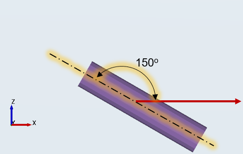
Figure 3. - Substitute the angles (0, -150, 0) in the respective matrices.
- Now multiply the 3 matrices .
- The resultant matrix will be your orientation matrix.
- After you specify this matrix in EDEM, it throws a warning message, but you can ignore it.
Part 1 - EDEM Simulation
Start Altair EDEM from the Windows start menu by clicking .
Open the EDEM Input Deck
-
In the dialog, browse to your problem directory and open the
cylinder.dem file.
The geometry and the materials are loaded.
Figure 4.
Review the Bulk Material and Particle Shape
In this step, you will define the material models for the bar and sphere-shaped particles.
-
Click cylinder and verify that the properties are set as
shown below.
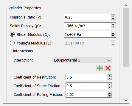
Figure 5. -
Click Properties under New particle 1.
Observe that the particle shape is created using multiple spheres aligned along the x-axis.Note: When defining non-spherical shapes, you need to make sure that the principal axis of the particle is aligned with the x-axis, as shown in the figure below.
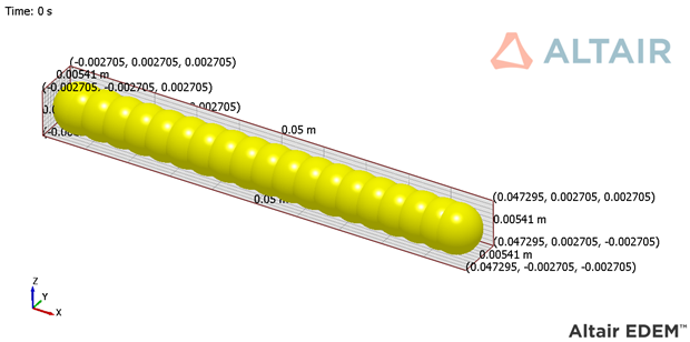
Figure 6.The length (L) and diameter (D) of the particle are 0.05 m and 0.00541 m respectively. Therefore, the aspect ratio (= L/D) of the particle is 9.242.
-
Observe the mass and volume of the particle in the Creator Tree.
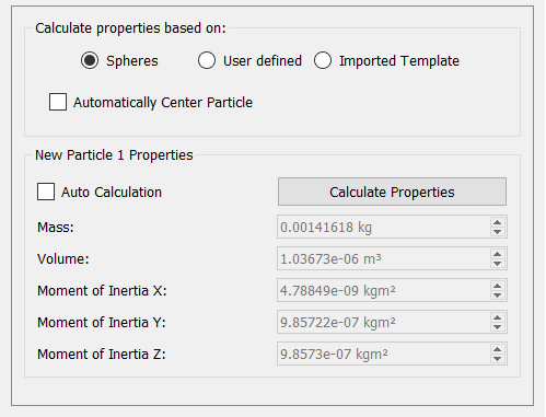
Figure 7.
Define Geometries and Factories
-
Click Tank and verify that the type is set to
Physical.
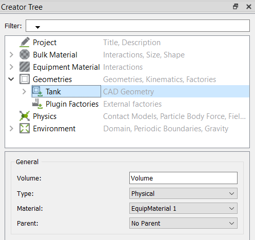
Figure 8. -
Verify that the Factory Type is set to static and set the particle generation
parameters as shown in the figure below.
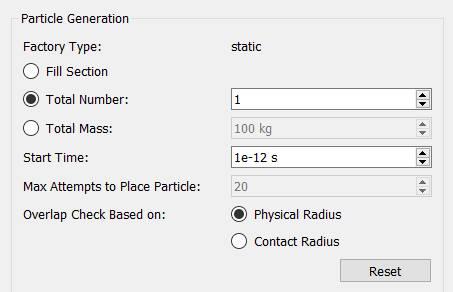
Figure 9. -
Under Parameters, set the Position option to cubic and
click
 .
.
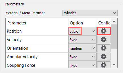
Figure 10. -
In the dialog, enter the position parameters as shown in the figure below then
click OK.
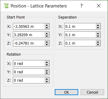
Figure 11. -
Under Parameters, set the Orientation option to fixed
and click .
-
Enter the values for the orientation matrix as shown in the figure below.
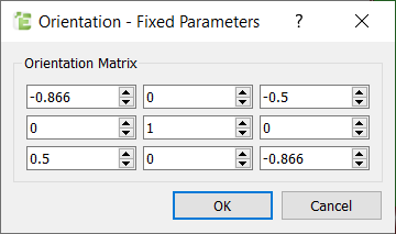
Figure 12.
Define the Environment
In this step, you will define the extents of the domain for the EDEM simulation and the direction of gravitational acceleration.
Define the Simulation Settings
-
Click
 in the top-left corner to go to
the EDEM Simulator tab.
in the top-left corner to go to
the EDEM Simulator tab.
-
Set the Selected Engine to CPU Solver and set the Number
of CPU Cores based on availability.
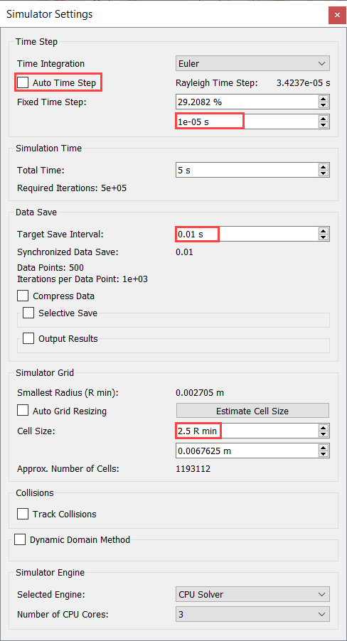
Figure 13.
Part 2 - AcuSolve Simulation
Start HyperWorks CFD and Open the HyperMesh Database
-
From the Home tools, Files tool group, click the Open Model tool.

Figure 14.The Open File dialog opens.
Validate the Geometry
The Validate tool scans through the entire model, performs checks on the surfaces and solids, and flags any defects in the geometry, such as free edges, closed shells, intersections, duplicates, and slivers.
Figure 15.
Set Up Flow
Set the General Simulation Parameters
-
From the Flow ribbon, click the Physics tool.

Figure 16.The Setup dialog opens. -
In the Material Library dialog, select EDEM 2 Way
Multiphase, switch to the My Materials
tab, then click
 to add a new material model.
-
Click the table icon beside the drag coefficient model drop-down.
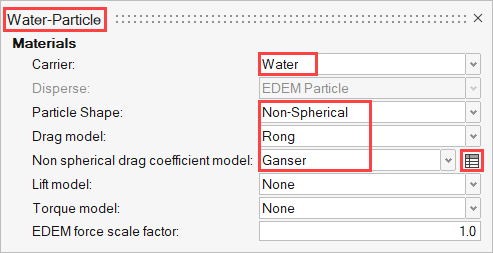
Figure 17. -
In the new dialog, enter the values for Aspect Ratio and Volume as shown in the
figure below.
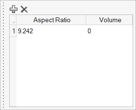
Figure 18.Note: Since you have only a single type of particle in this simulation, you don’t need to specify the volume of the particle. But, in the case of multiple particles, the volume of each particle should be specified, which can be obtained from EDEM. -
Set the Torque model to Pitching Rotational
Torque.
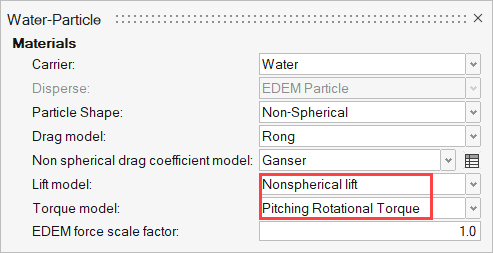 Figure 19.
 -
Set the Pressure scale to Absolute.
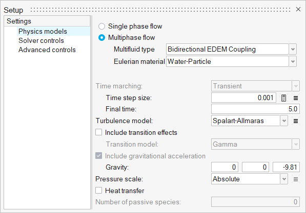
Figure 20. -
Click the Solver controls setting and set the Maximum
stagger iterations to 2.
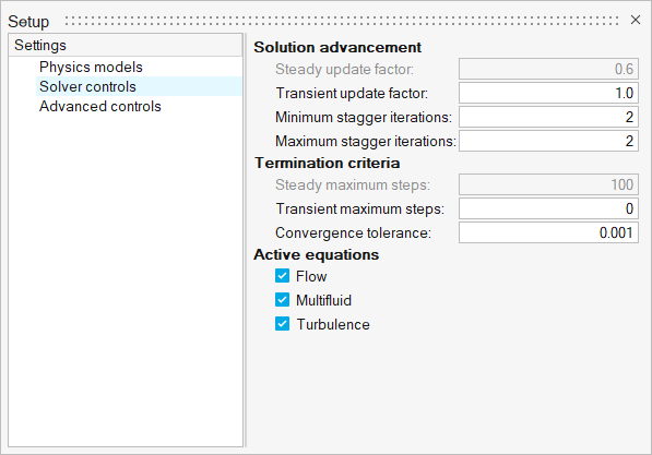
Figure 21.
Assign Material Properties
-
From the Flow ribbon, click the Material tool.

Figure 22. -
On the guide bar, click
 to exit
the tool.
to exit
the tool.
Define Flow Boundary Conditions
Since the domain doesn’t have any openings, there is no need to explicitly define a surface boundary condition as HyperWorks CFD assigns a no-slip wall boundary condition to all the surfaces by default.
Generate the Mesh
-
From the Mesh ribbon, click the
Volume tool.

Figure 23.The Meshing Operations dialog opens. -
Deactivate Curvature-based surface refinement then click
Mesh.
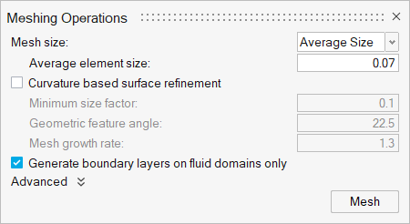
Figure 24.
Define Nodal Outputs
Once the meshing is complete, you are automatically taken to the Solution ribbon.
-
From the Solution ribbon, click the Field tool.

Figure 25.The Field Output dialog opens. -
Set the Time step interval to 0.01.
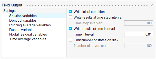
Figure 26.
Submit the Coupled Simulation
-
Start the coupling server by clicking Coupling Server in
EDEM.
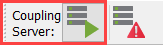
Figure 27.Once the Coupling server is activated, the icon changes.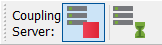
Figure 28. -
From the Solution ribbon, click the Run tool.

Figure 29.The Launch AcuSolve dialog opens. -
Click Run to launch AcuSolve.
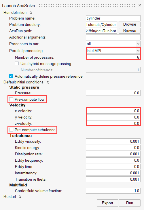
Figure 30.Once the AcuSolve run is launched, the Run Status dialog opens. -
In the dialog, right-click on the AcuSolve run and
select View log file.
If the coupling with EDEM is successful, that information is printed in the log file.
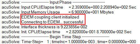
Figure 31.Once the simulation is complete, the summary of the run time is printed at the end of the log file.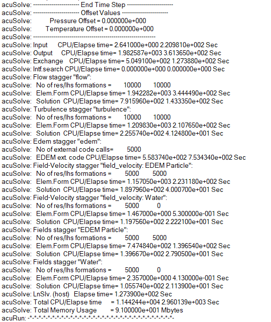
Figure 32.
Analyze the Results
AcuSolve Post-Processing
-
In HyperWorks CFD, right-click on the AcuSolve run in the Run Status
dialog and select Visualize results.
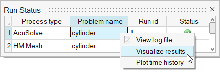
Figure 33.The results are loaded in the Post ribbon. -
Click the Slice Planes tool.

Figure 34. -
Select the x-z plane as highlighted in the figure below.
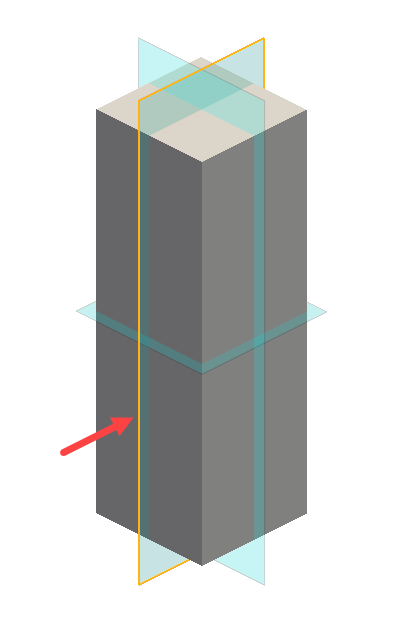
Figure 35. -
In the slice plane microdialog, click
 to
create the slice plane.
to
create the slice plane.
-
Click
 and set the Colormap name to Rainbow
Uniform.
and set the Colormap name to Rainbow
Uniform.
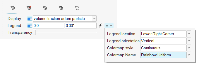
Figure 36. -
Click and set the Vector length to
Uniform.
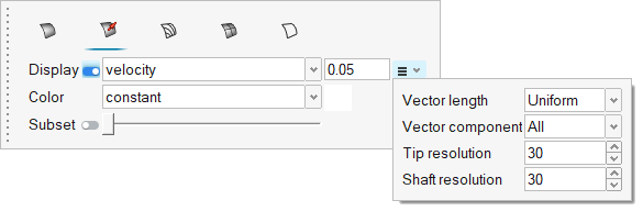
Figure 37. -
Click on the guide bar.
-
In the Post Browser, turn off the visibility of
Flow Boundaries by clicking on its icon.
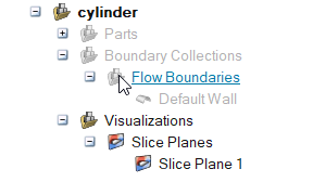
Figure 38. -
Select the Left face on the view cube to align the model
to the x-z plane.
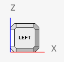
Figure 39. -
Click
 on the animation toolbar to view the
animation.
on the animation toolbar to view the
animation.
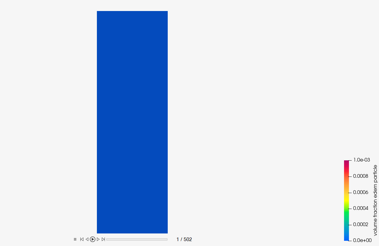
Figure 40.
EDEM Post-Processing
-
Once the EDEM simulation is complete, click
 in the top-left corner to go to
the EDEM Analyst tab.
in the top-left corner to go to
the EDEM Analyst tab.
-
Verify that the Display Mode is set to Filled and set
the Opacity to 0.2.
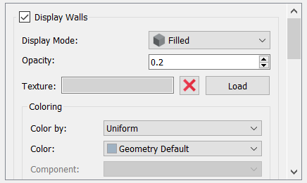
Figure 41. -
Click Apply All.
Figure 42. -
On the menu bar, set the time to
0 by clicking:

Figure 43. -
Set the View plane to + Y.
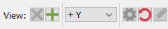
Figure 44. -
In the Viewer window, set the Playback Speed to 0.2x and
then click
 to play the particle flow animation.
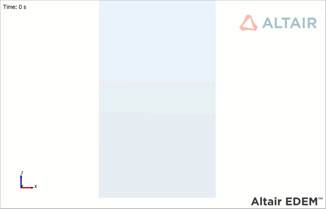
Figure 45.Observe that the particle rotates and translates as it falls down. Without lift and torque, you will not see this phenomenon.
Summary
In this tutorial, you learned how to set up and run a basic AcuSolve-EDEM bidirectional (two-way) coupling problem with non-spherical particles. You learned how to create particles in EDEM with a specific orientation and position. Next, you set up the AcuSolve model to consider the effect of the lift and torque forces. Once the simulation is complete, you learned how to post-process the AcuSolve results using HyperWorks CFD and EDEM.