HG-3010: Working with Complex Plots
In this tutorial, you will learn how to create complex plots from a data file and add and edit complex data curves by using mathematical functions.
The Build Plots panel can be accessed in one of the following ways:
- Click the Build Plots icon from the toolbar,

- From the menu, bar select
The Build Plots panel constructs multiple curves and plots from a single data file. Curves can be overlaid in a single window or each curve can be assigned to a new window. Individual curves are edited using the Define Curves panel.
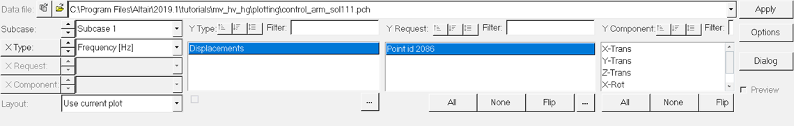
Figure 1.
The Define Curves panel can be accessed in one of the following ways:
- Click the Define Curves panel icon,
 , from the toolbar
 - From the menu bar select
Existing curves can be edited individually and new curves can be added to the current plot using the Define Curves panel. The Define Curves panel also provides access to the program's curve calculator.
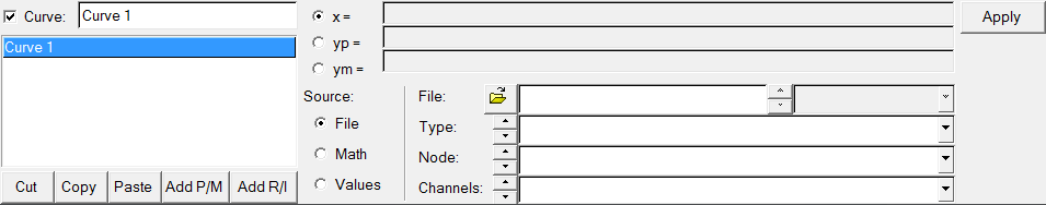
Figure 2.
Build a Complex Data Curve from a Data File
-
From the plot type menu, select Complex Plot
 .
.
-
Enter the Build Plots panel
 .
.
-
Click Apply to create the complex curves.
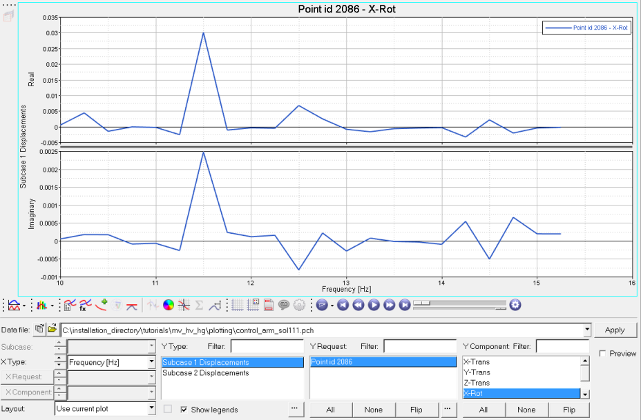 Figure 3.
Apply the Inverse Fast Fourier Transform (ifft) Math Function to the Complex Data Curve
-
Change the current window layout of page 1 to a two-window layout
 .
.
-
Enter the Define Curves panel,
 .
.
-
Click Apply to create the XY data curve.
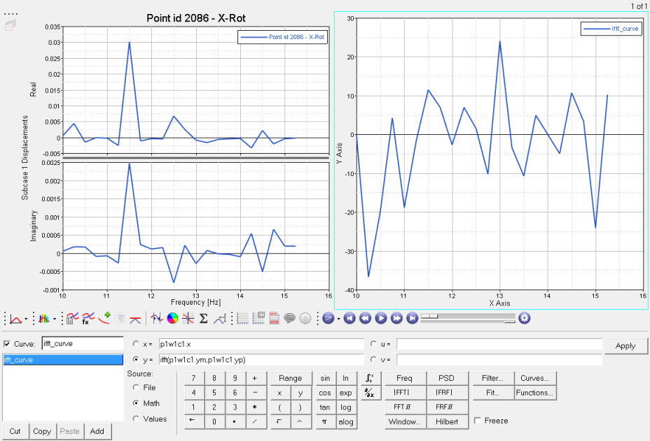 Figure 4.
Create a Complex Data Curve of Frequency Versus Displacement for Subcase Two, Node 2086, X-Rotation
-
Enter the Build Plots panel, .
-
Click Apply to create the complex curves.
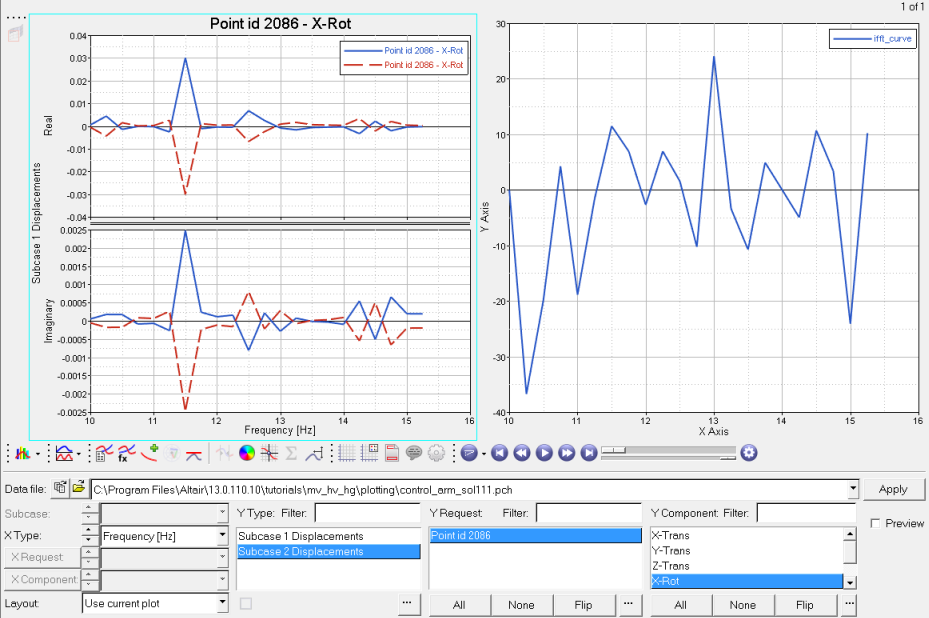 Figure 5.
Subtract the Subcase Two Curve from the Subcase One Curve
-
Change the current window layout for page 1 to a three-window layout,
 .
.
-
Click Apply to create the complex curve.
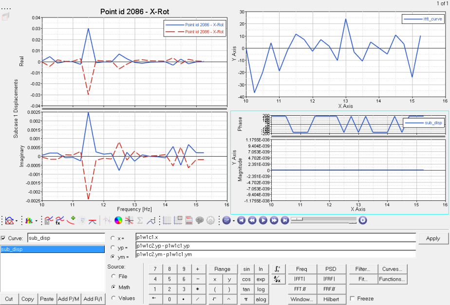 Figure 6.