HS-3005: Export Fit Models to Excel

1. Start a new study in the following ways:
   • From the menu bar, click File > New.
   • On the ribbon, click .
2. In the Add Study dialog, enter a study name, select a location for the study, and click OK.
3. Go to the Define Models step.
4. Add an Internal Math model.
   1. Click Add Model.
   2. In the Add dialog, select Internal Math and click OK.
5. Go to the Define Input Variables step.
6. Click Add Input Variable to add two input variables.
7. Change the input variables' Lower Bounds, Initial, and Upper Bounds to the values shown in Figure 1.

   
   
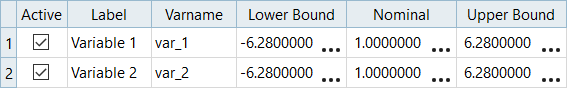
   Figure 1.

1. Go to the Test Models step.
2. Click Run Definition.
   An approaches/setup_1-def/ directory is created inside the study directory. The approaches/setup_1-def/run__00001/m_1 directory contains the input file, which is the result of the nominal run.

In this step you will create the output responses.

1. Go to the Define Output Responses step.
2. Click Add Output Responses.
3. In the Expression column of Response 1, enter sin(var_1)*cos(var_2).

   
   
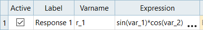
   Figure 2.

4. Click Evaluate to extract the response values.

1. Add a DOE.
   1. In the Explorer, right-click and select Add from the context menu.
   2. In the Add dialog, select DOE and click OK.
2. Go to the DOE 1 > Specifications step.
3. In the work area, set the Mode to Hammersley.
4. In the Settings tab, change the Number of Runs to 50.
   Note: The large number of runs relative to the number of input variables is chosen to capture the highly non-linear nature of the output response function. This model is simple to evaluate, therefore the computational cost of the evaluation is not an important consideration in this example.

   
   
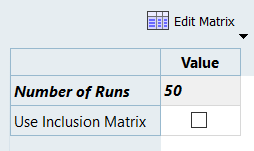
   Figure 3.

5. Click Apply.
6. Go to the DOE 1 > Evaluate step.
7. Click Evaluate Tasks.

In this step, you will run a Radial Basis Function (RBF) fit.

1. Add a Fit.
   1. In the Explorer, right-click and select Add from the context menu.
   2. In the Add dialog, select Fit and click OK.
2. Import matrix.
   1. Go to the Fit 1 > Specifications step.
   2. Click Add Matrix.
   3. In the work area, set Matrix Source to Doe 1 (doe_1).
   4. Click Apply.
3. Define specifications.
   1. In the work area, Fit Type column, select Radial Basis Function.
   2. Click Apply.

   
   
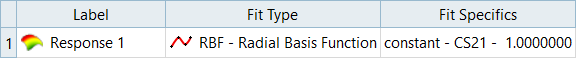
   Figure 4.

4. Evaluate tasks.
   1. Go to the Fit 1 > Evaluate step.
   2. Click Evaluate Tasks.
5. Go to the Fit 1 > Post-Processing step.
6. Visualize the response surface as a function of two input variables.
   1. Click the Trade-Off tab.
   2. In the Inputs pane, select the X Axis checkbox for Variable 1 and the Y Axis checkbox for Variable 2.

      
      
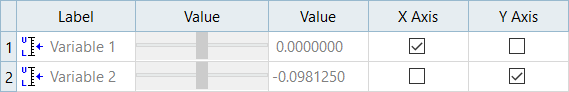
      Figure 5.

   3. In the Outputs pane, click and adjust the plotting resolution of the display to include 25 samples.

      
      
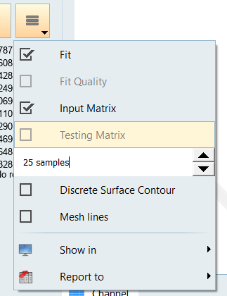
      Figure 6.

   4. Visually examine the plotted response surface to inspect the quality of the approximation to the original sinusoidal function.

      
      
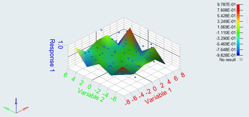
      Figure 7.

7. In the Trade-Off tab, interactively predict output response values as a function of the input variables.
   1. In the Inputs pane, clear the X Axis and Y Axis checkboxes.
   2. In the Inputs pane, modify the values of each input variable by moving the slider in the first Value column, or by entering values in the second Value column.
      The predicted output response value in the Value column of the Outputs table is adjusted.

      Note: The shaded spark lines in the Value cell indicate the relative value of the predicted output response with respect to the minimum and maximum of the sample. The marker at the bottom of the cell references the value of the predicted output response at the nominal values of the input variables.

      
      
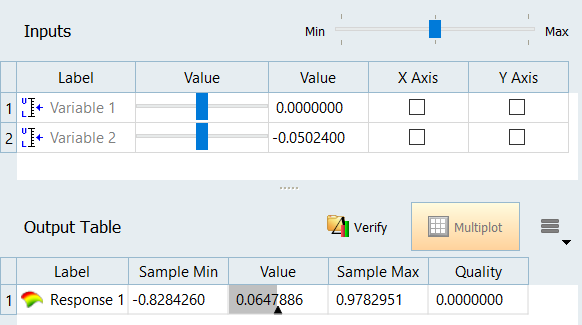
      Figure 8.

8. Export Excel report for Fit.
   1. Go to the Fit 1 > Report step.
   2. Click the HyperStudy Spreadsheet checkbox.
   3. Click Create Report.
      An Excel report is generated and opened in Excel.
   4. In the Excel report, click the Trade-Off tab.
      Note: The structure and functionality of this tab is a reflection of the corresponding Trade-Off tab within HyperStudy. You can adjust the input variable values on the right-hand side, and the predicted output response values are updated and displayed on the left-hand side.
   5. To verify that the same values occur in the output response prediction columns for the same set of input variables, simultaneously adjust the values within HyperStudy and the Excel report.

   
   
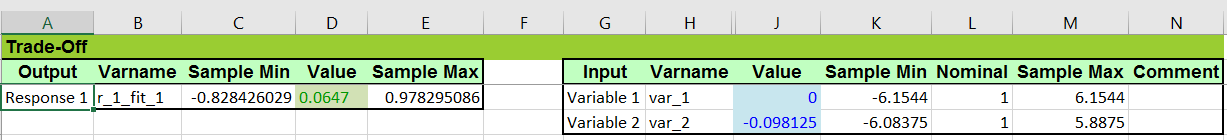
   Figure 9.