HS-3010: Fuselage Sizing Trade-Off using Categorical Variables
Learn how to create a Fit in order to investigate the relative effect of the variable on the identified output responses, and identify a combinations of variables that were not explicitly simulated.
- Continuous variables
- Thickness of floor
- Category variables
- Cross sections of the frames
- Load cases
- Free-free normal modes case
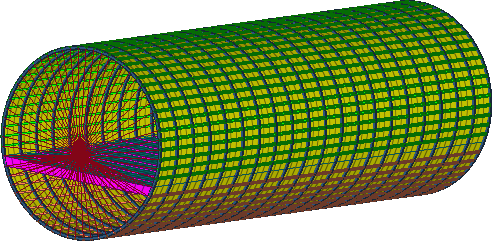
Figure 1.
Perform the Study Setup
-
Start a new study in the following ways:
- From the menu bar, click .
- On the ribbon, click
 .
.
-
Add a Parameterized File model.
-
From the Directory, drag-and-drop the fuselage.tpl
file into the work area.
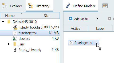
Figure 2.
-
From the Directory, drag-and-drop the fuselage.tpl
file into the work area.
-
Modify input variable mode.
-
In the Mode column, change the input variables defined as Discrete to
Categorical.
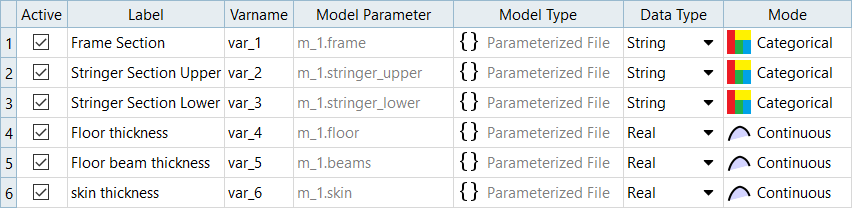
Figure 3.
-
In the Mode column, change the input variables defined as Discrete to
Categorical.
Perform Nominal Run
Create and Evaluate Output Responses
-
Create the Mass output response.
-
Define the following options:
- Type: Mass
- Request: Mass
- Component: Value
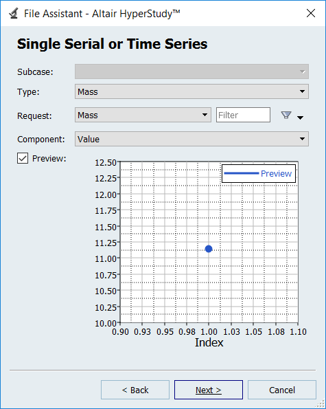
Figure 4. -
Click Finish.
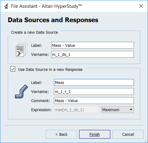
Figure 5.
-
Define the following options:
-
Create the Torsional rotation output response, which will have a z-direction of
node 8196 (loading point).
-
In the Expression field for Torsional rotation, edit the expression to
be max(m_1_ds_5)*180/3.14.
This expression converts the rotation from radians to degrees.

Figure 6.
-
In the Expression field for Torsional rotation, edit the expression to
be max(m_1_ds_5)*180/3.14.
Run DOE
-
Edit run matrix.
-
In the top, right of the work area, select .
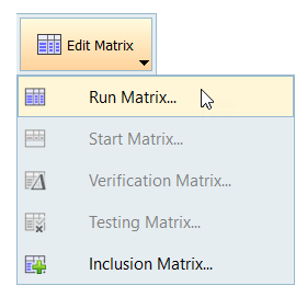
Figure 7. -
Review the imported run data and click Apply.
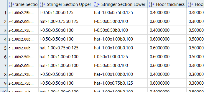
Figure 8.
-
In the top, right of the work area, select .
-
Review Pareto plot.
-
Click
 (Multiplot).
The relative effect of a input variable can vary from output response to output response. The most influential input variables when analyzing frequency output responses are Frame Section and Stringer Section Upper. In contrast, the most influential input variables when analyzing the two stiffness conditions are Skin thickness and Stringer Section Upper.
Some input variables can have no effect on output responses. Floor beam thickness has minimal effect on any of the output responses, which indicates that you may want to consider removing this input variable from the analysis.
In a Pareto plot, the effect of input variables on output responses does not measure sensitivity but rather absolute change. Floor thickness has a major effect on Volume. This effect is not a derivative, but a measure of the possible increase over the range of the input variables (the range is the difference between the upper and lower bounds). The floor has a large area and the thickness has very large bounds (+/-0.1 inches), therefore it can make a dramatic impact on Volume as the input variables move through the available space.
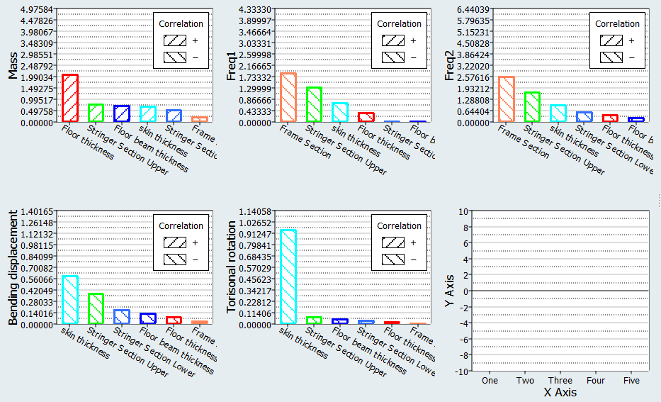
Figure 9. -
Click
Run Least Squares Regression Fit
-
Define specifications.
- In the work area, Fit Type column, select Least Squares Regression for all output responses.
- Click Apply.
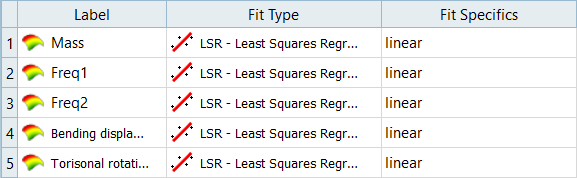
Figure 10. -
Assess the accuracy of the Fit.
-
Select the Mass output response.
The R-Square and R-Squared Adjusted values for Mass are close to 1.00, which indicates the model almost perfectly predicted the known values.
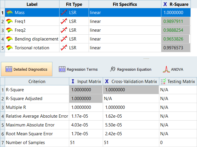
Figure 11.
-
Select the Mass output response.