HS-2000: DOE Method Comparison: Arm Model Study
Learn how to set up DOEs using different methods and then compare methods for accuracy and efficiency.
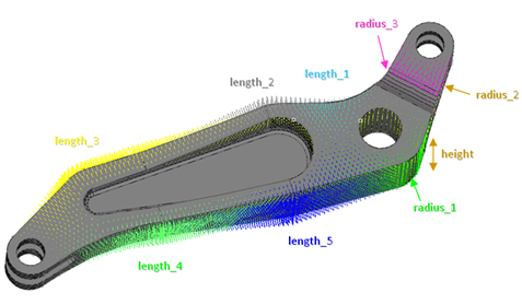
- Shape input variables
- Length1: Lower Bound = -0.5, Initial Bound = 0.0, Upper Bound = 2.0
- Output responses
- Volume (Nominal design volume 1.7667e6 mm3)
You will study the results from different parameter screening DOEs. For each screening, only the results obtained on the Max_stress output response will be reviewed using Pareto plot, Interactions, and Ordination displays.
- A Full Factorial provides excellent resolution but typically requires an exceedingly large number or runs.
- A Fractional Factorial with a Resolution III confounds main effects with interactions; results could be inaccurate if interactions are significant.
- A Fractional Factorial with a Resolution IV main effects are not confounded, but interactions are confounded with each other.
- A Fractional Factorial with a Resolution V main effects and interactions are not confounded.
Perform the Study Setup
In this step you will start from an already morphed model. The shape variables are already exported for HyperStudy and a template is created.
-
Start a new study in the following ways:
- From the menu bar, click .
- On the ribbon, click
 .
.
-
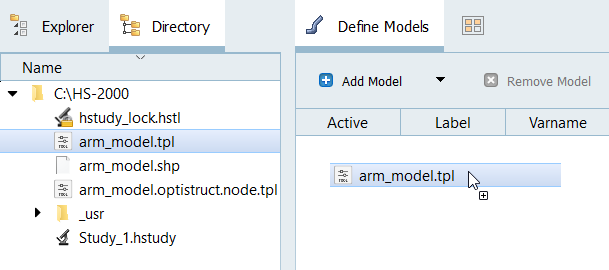
Add a Parameterized File model.
-
From the Directory, drag-and-drop the
arm_model.tpl file into the work area.
Figure 3.
-
From the Directory, drag-and-drop the
arm_model.tpl file into the work area.
Perform Nominal Run
Create and Evaluate Output Responses
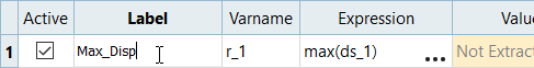
In this step you will create three output responses: Max_Disp, Max_Stress, and Volume.
-
Create the Max_Disp output response.
-
Define the following options, then click
Next.
- Set Subcase to Subcase 1 (SUBCASE1).
- Set Type to Displacement (Grids).
- For Request (Start - End), enter N27099 - N40946.
- For Components, select MAG.
Figure 4.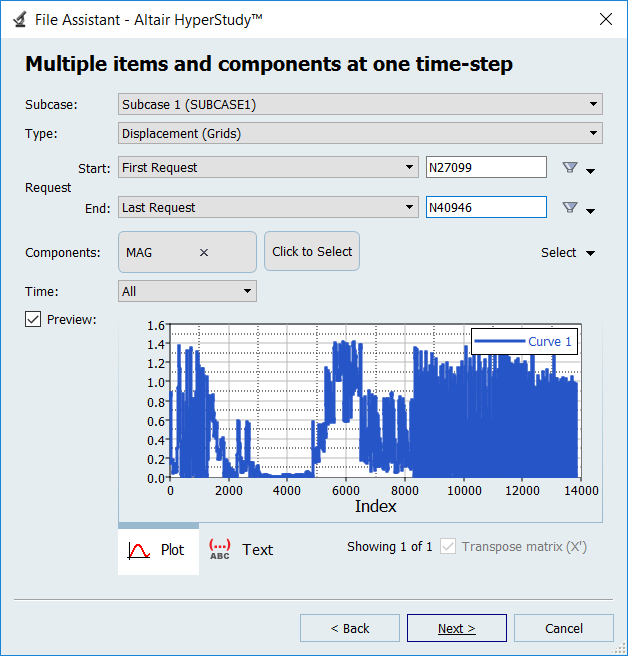
-
Click Finish.
The Max_Disp output response is added to the work area.Figure 5.
-
In the work area, Label the second output response
Max_Disp.
Figure 6.
-
Define the following options, then click
Next.
-
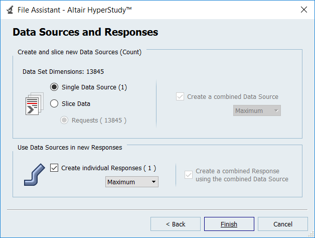
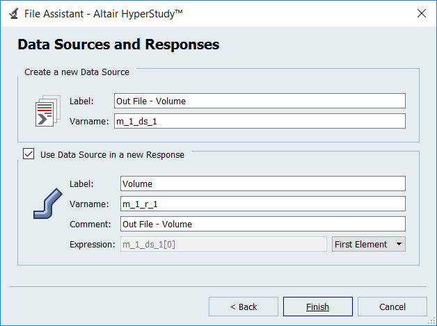
Create the Volume output response.
-
Click Finish.
The Volume output response is added to the work area.Figure 7.
-
Click Finish.
-
Minimize the size of the result files in the study directory.
- Click the Data Sources tab.
- Clear the Retain checkbox for Displacement (Grids) MAG and Element Stresses (3D) vonMises (2D & 3D) data sources.
Figure 8.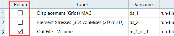
Run Full Factorial DOE
In this step you will create a Full Factorial DOE, and set the shape variables to two levels.
-
Define specifications.
-
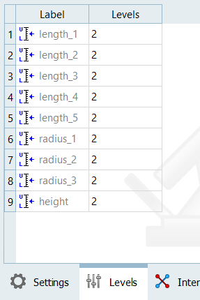
Click the Levels tab, and verify that the number
of levels for each input variable is 2.
Using nine shape variables with two levels gives a full factorial plan made of 512 runs (2^9).Figure 9.
-
Click the Levels tab, and verify that the number
of levels for each input variable is 2.
-
Evaluate tasks.
-
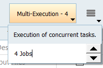
Above the Channel Selector, click
Multi-Execution and change the number of jobs
to 4.
Figure 10.
-
Above the Channel Selector, click
Multi-Execution and change the number of jobs
to 4.
-
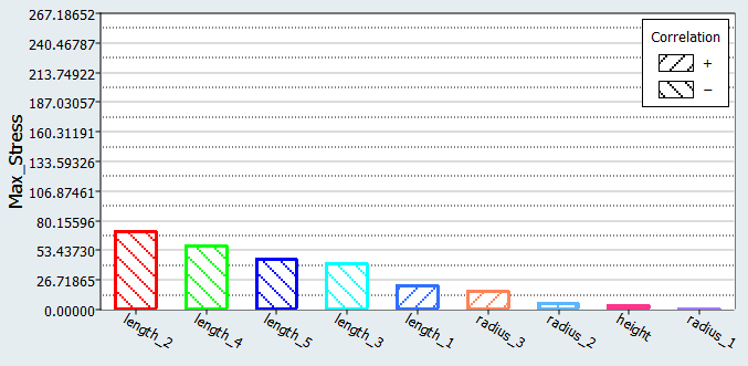
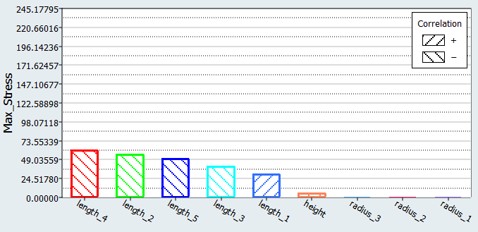
Click the Pareto Plot tab to view Pareto plots obtained
from the Full Factorial DOE (512 runs).
A Pareto Plot shows the ranked influence (highest to lowest) of the design variables on the response.
The 5 lengths have the largest influence, and the 3 radii have the least influence on Max_stress. The slope of the hashed lines (positive or negative) indicates a positive or a negative effect of a variable on the response. length_4, length_2, length_5, and length_3 have negative slopes, which indicates that if these variables increase, Max_stress will decrease. On the other hand, length_1 has a positive slope, which indicates that increasing length_1 increases Max_stress.Figure 11.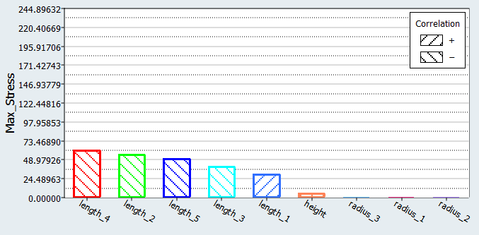
-
Click the Interactions tab to plot the interactions
between input variables.
An interaction is the failure of one variable to produce the same effect on a response at different levels of another variable. An interaction can be either positive or negative. The Interaction plot displays parallel lines if there is no interaction. The bigger the interaction is, the less parallel the lines will be.Looking at the Max_stress output response, you can see that several of the interactions are very small. You can still find instances with a true interaction, such as the interaction of length_5 and length_4. The effect of the variable length_4 on the output response Max_Stress is in the same direction regardless of the value of length_5, but the effect (magnitude) is much more important when length_5 is larger.Figure 12. Interaction between length_5 and length_4 on Max_Stress
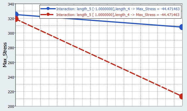 Figure 13. No interaction between length_1 and length_5 on Max_Stress
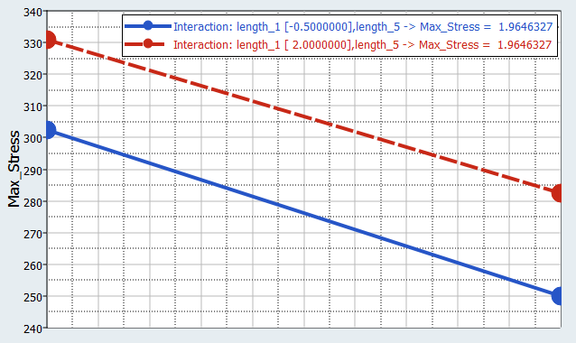
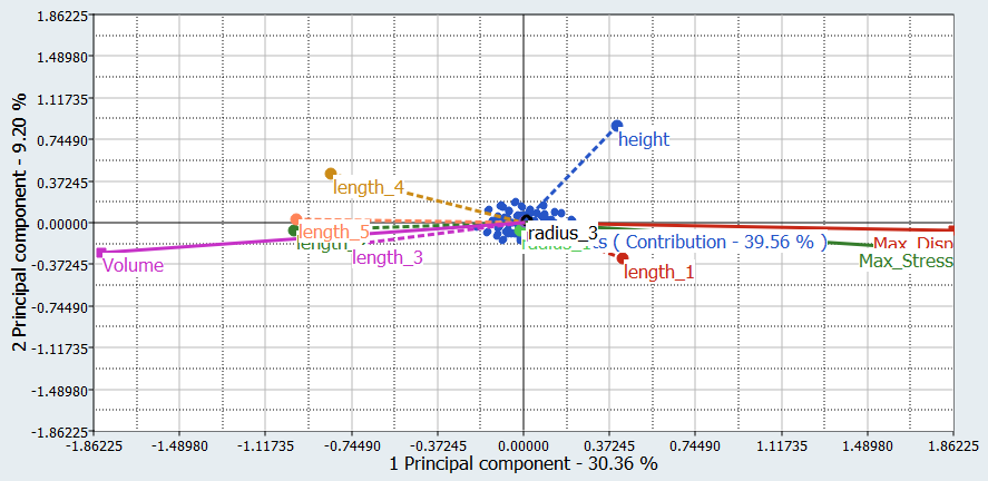
-
Click the Ordination tab to see the Principal Component
Analysis results.
Tip: If the 3D Scatter tab is not enabled, click
 (Show or Hide
Tabs), and select 3D Scatter from the Standard
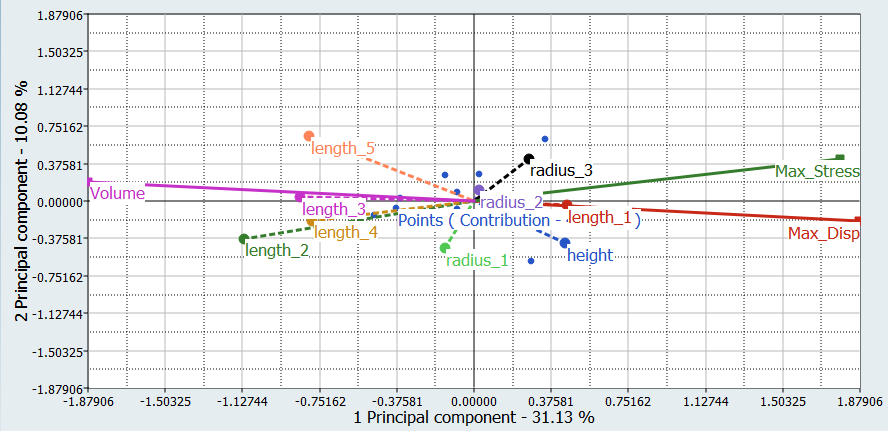
Tabs.Each input variable and output response in the biplot is represented by a line. Lines that point in the same direction have strong correlations (positive or negative depending on whether the lines point in the same or opposite directions). You can see that lengths 2, 3, 4, and 5 contribute the most to the volume value, and improve the structural performance the most along with height and length_1.Figure 14.
(Show or Hide
Tabs), and select 3D Scatter from the Standard
Tabs.Each input variable and output response in the biplot is represented by a line. Lines that point in the same direction have strong correlations (positive or negative depending on whether the lines point in the same or opposite directions). You can see that lengths 2, 3, 4, and 5 contribute the most to the volume value, and improve the structural performance the most along with height and length_1.Figure 14.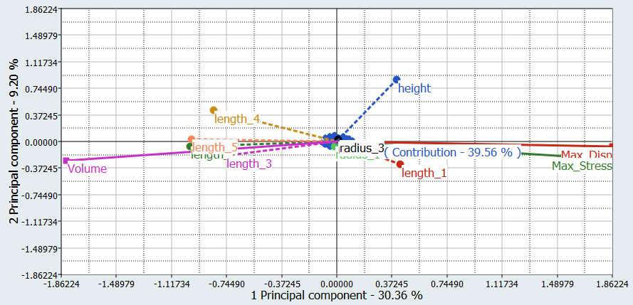
Run Fractional Factorial DOE with Resolution III
In this step you will set up a Fractional Factorial DOE, with resolution III and the same levels as the previous Full Factorial DOE.
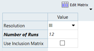
Use the nine input variables with two levels, without turning on any interaction, leads to a 12 run Fractional Factorial plan.
-
Define specifications.
-
In the Settings tab, set Resolution to
III.
Figure 15.
-
In the Settings tab, set Resolution to
III.
-
Click the Pareto Plot tab to view Pareto plots on
Max_stress obtained from the Fractional Factorial III DOE (12 runs).
Compared to the Pareto plot from the Full Factorial, several differences can be observed.
The rank of variables is not the same; for instance, length_4 is the most influential input variable in the Full Factorial, whereas length_2 is the most influential input variable in the Fractional Factorial III.
The effect of length_5 has decreased, while the effects of the three radii has significantly increased, especially the effects of radius_3 and radius_1.Figure 16. Full FactorialFigure 17. Fractional Factorial III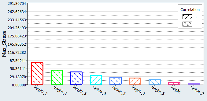
-
Click the Interactions tab to plot the interactions
between input variables.
Compare the interaction between length_1 and length_3 on Max_stress. The results provided from the Full Factorial and Fractional Factorial III are quite different. The Full Factorial establishes the real interactions, while the Fractional factorial III detects confounded interactions inaccurately.Figure 18. Full Factorial
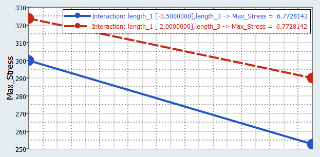 Figure 19. Fractional Factorial III
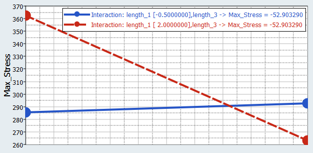
-
Click the Ordination tab to see the Principal Component
Analysis results obtained with the Fractional factorial III.
In the Full Factorial, you can see that length_2, length_3, and length_5 are correlated to the Volume output response. In the Fractional Factorial III, the relationship is not as clear. In the Fractional Factorial III, the lines representing length_2, length_3, length_5, and Volume are not as collinear as they are in the Full Factorial.Figure 20. Full FactorialFigure 21. Fractional Factorial III
Run Fractional Factorial DOE with Resolution IV
In this step you will set up a Fractional Factorial DOE with Resolution IV. Using the nine input variables with two levels, without turning on any interaction, leads to a 24 run Fractional Factorial plan.
-
Click the Pareto Plot tab to view Pareto plots on
Max_stress obtained from the Fractional Factorial IV DOE (24 runs).
Compared to the results obtained from the Full Factorial, you can see that the places of length_2 and length_4 have been inversed in the ranking, but the rest of the information is quite similar.Figure 22. Full FactorialFigure 23. Fractional Factorial IV
Run Fractional Factorial DOE with Resolution V
In this step you will set up a Fractional Factorial DOE with Resolution V. Using the nine input variables with two levels, without turning on any interaction, leads to a 128 run Fractional Factorial plan.
-
Click the Pareto Plot tab to view Pareto plots on
Max_stress obtained from the Fractional Factorial V DOE (128 runs).
The results obtained from both DOE methods are the same, but the number of runs for the Fractional Factorial V is only 1/4th of the runs for the Full Factorial.Figure 24. Full FactorialFigure 25. Fractional Factorial V
-
Click the Ordination tab to see the Principal Component
Analysis results obtained from the Fractional factorial V.
There are no differences between the results obtained from the Full Factorial and the Fractional Factorial V.Figure 26. Full FactorialFigure 27. Fractional Factorial V
Comparison
Conclusions on the screened output responses are summarized for the four DOE methods.
In this tutorial, you focused on the Max_Stress output response, but the same steps should be applied for all output responses.
| Full Factorial | Fractional Factorial V | Fractional Factorial IV | Fractional Factorial III | |
|---|---|---|---|---|
| Number of runs | 512 | 128 | 24 | 12 |
| Max_Stress | Remove all radii and height | Remove all radii and height | Remove radii 1, 2 and height | Remove radius 2 and height |
| Max_Disp | Remove all radii | Remove all radii | Remove all radii | Remove all radii |
| Volume | Remove all radii | Remove all radii | Remove all radii | Remove all radii |
| Conclusion | Remove all radii | Remove all radii | Remove radii 1 and 2 | Remove radius 2 |