HS-2210: Principle Component Analysis of a Cantilever Ibeam
Learn perform a Principle Component Analysis of a cantilever ibeam using a D-Optimal DOE.
Before you begin, copy the model files used in
this tutorial from <hst.zip>/HS-2210/ to your working
directory.
Perform the Study Setup
-
Start a new study in the following ways:
- From the menu bar, click .
- On the ribbon, click
 .
.
-
Add a Parameterized File model.
-
From the Directory, drag-and-drop the ibeam.tpl
file into the work area.
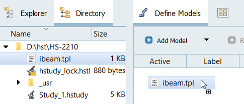
Figure 1.
-
From the Directory, drag-and-drop the ibeam.tpl
file into the work area.
Perform Nominal Run
Create and Evaluate Output Responses
-
Create the Iy output response for the y-axis moment of inertia.
-
Define the following options, and then click
Next.
- Set Type to Output.
- Set Request to Iy.
- Set Component to Value.
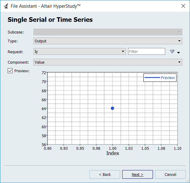
Figure 2. -
Click Finish.
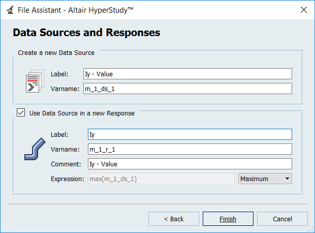
Figure 3.
-
Define the following options, and then click
Next.
Run D-Optimal DOE
-
In the Settings tab, change the Number of Runs to
13.
This is 2 more runs than the minimum required value.
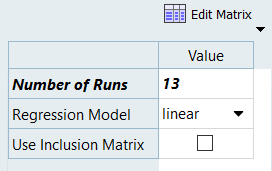
Figure 4. -
Click the Ordination tab.
The biplot is interpreted by looking at the relationship between the lines that each represent one input variable or output response. The Displacement and Iy output responses show a strong negative correlation because they are aligned, but pointing in opposite directions. The displacement and Iy are also not at all correlated to the input variable web thickness, indicated by the orthogonality. Similar strong positive correlations are seen between the frequency and height or the volume, Iz, and flange length.
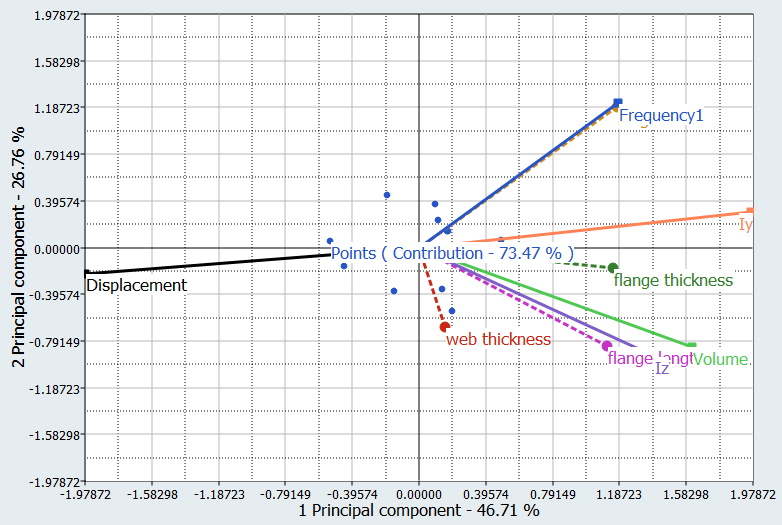
Figure 5.