HS-2005: DOE Study of a Cantilever Beam using Templex
Learn how to run a simple DOE study on a cantilever beam to examine the influence of the length, width, and height of the beam on its volume, maximum bending stress, and deflection.
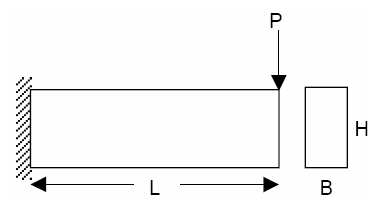
Figure 1. Cantilever Beam
{parameter(L,"Length",50,50,100)}
{parameter(B,"Width",2.5,2.5,5)}
{parameter(H,"Height",5,5,10)}
{P = 100}
{E = 2e11}
{M = P*L}
{c = H/2}
{I = (B*H^3)/12}
{MAX_STRESS = (M*c)/I}
{MAX_DISP = (P*L^3)/(3*E*I)}
{VOLUME = B*H*L}
{MAX_STRESS}
{MAX_DISP}
{VOLUME}
Perform the Study Setup
In this step you will add a study and load the input file into HyperStudy.
The input variables for the DOE study (length, width, and height) are selected as factors. A nominal run is performed (with Templex as the solver), and the output responses for the DOE study are selected (in this case: volume, max. stress, and max. displacement).
-
Start a new study in the following ways:
- From the menu bar, click .
- On the ribbon, click
 .
.
-
Add a Parameterized File model.
-
From the Directory, drag-and-drop the beam.tpl
file into the work area.
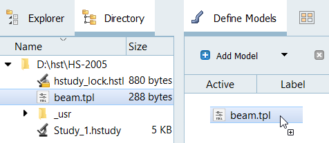
Figure 2.
-
From the Directory, drag-and-drop the beam.tpl
file into the work area.
Perform Nominal Run
Create and Evaluate Output Responses
In this step you will create three output responses: Max_Stress, Max_Disp, and Volume.
-
Create the Max_Stress output response.
-
Define the following options, then click
Next.
- Set Type to Unknown.
- Set Request to Block 1.
- Set Component to Column 1.
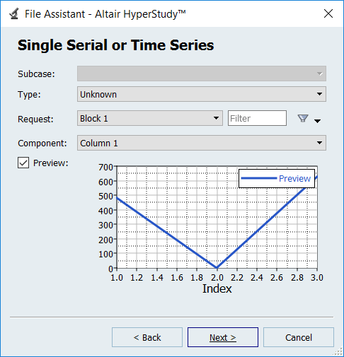
Figure 3. -
Click Finish.
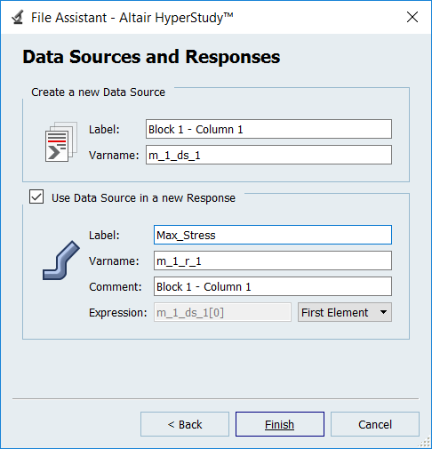
Figure 4.
-
Define the following options, then click
Next.
-
In the work area, Expression field, edit expressions.
- For Max_Disp, after m_1_ds_2, change [0] to [1].
- For Volume, after m_1_ds_3, change [0] to [2].
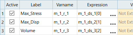
Figure 5.
Run DOE
In this step you will set up a DOE approach through the selection of a DOE matrix and input variables.
Input variables can either be controlled or uncontrolled. In this exercise, a full factorial DOE matrix is considered. This provides the main effect of the input variables and their interactions with one another for selected output responses. The length, width, and depth of the input variables are introduced as controlled and their effects are studied for the following output responses: maximum stress, maximum displacement, and volume.
-
Review the main effect of each controlled parameter on a selected output
response.
- Click the Linear Effects tab.
-
Above the Channel selector, click
 to plot the
linear effects.
to plot the
linear effects.
- Use the Channel selector to select the all input variables and the Max_Stress output response.
Review the effects of a single input variable on an output response, or multiple input variables on an output response.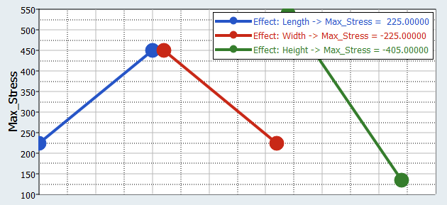
Figure 6.As illustrated in Figure 6, as the length increases from 50 to 100 units, the max stress increases from 225 to 450. Increasing the width from 2.5 to 5 units decreases the max stress by the same amount. The contributions for max stress from both length and width are identical. Increasing the height from 5 to 10 units decreases the max stress by a larger extent (from 530 to 130). It is clear that for the max stress output response, height has a larger main effect than length or width.Input Variable Max_Stress - Lower Bound Max_Stress - Upper Bound Length 225 450 Width 450 225 Height 540 135 -
Click the Distribution tab to review a histogram of Max
Stress.
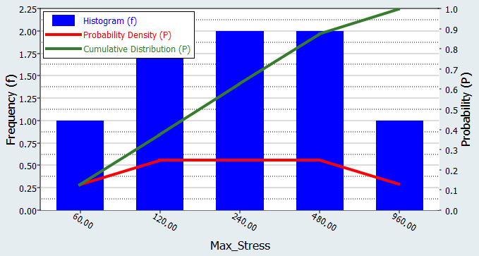
Figure 7.
Run Fit for Regression Equation
In this step you will create approximations for the DOE study.
A first order regression equation for each output response (Max Stress, Max disp, and Volume) is created based on the DOE study. Since the input variables are of two levels, only the first order equation can be generated.
-
Import matrix.
- Go to the step.
- Click Add Matrix.
- In the work area, set Matrix Source to DOE 1 (doe_1).
- Click Import Matrix.

Figure 8. -
Define specifications.
- Go to the step.
- In the work area, Fit Type column, select Least Squares Regression (LSR) for all output responses.
- Click Apply.
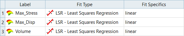
Figure 9. -
Click the Residuals tab.
The Residuals table displays the difference between the output response value from the solver and the output response value calculated from the regression equation. This table can also be used to determine which runs are generating more errors in the regression model. The % error column shows that the predicted output response is not close to the observed value. The % error can be reduced if more levels are chosen for example, using a three-level design in this exercise.
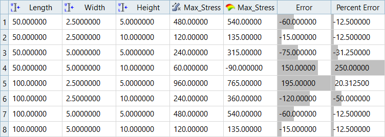
Figure 10. -
Plot output responses vs. input variables.
- Click the Trade-Off tab.
- In the Inputs pane, select the X Axis and Y Axis checkboxes for Length.
- Using the Channel selector, selector Max_Stress.
- Review the plot in the Outputs pane.
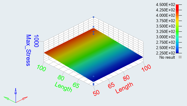
Figure 11.